Why do some long run average cost curves are U-shaped but some are L-shaped? Differentiate with the reasons.
Why do some long run average cost curves are U-shaped but some are L-shaped? Differentiate with the reasons.
(किनकुनै दीर्घकालिन औसत लागतवक्र U आकारका हुन्छन् तरकुनै दीर्घकालिनऔसत लागतबक्र L आकारका हुन्छन् ? कारणहरु सहित छुट्ट्याउनुहोस् ।)
Question from
Tribhuvan University MGT 207 · Microeconomics for Business 1 paper
Solution
The long-run average cost (LAC) curve shows the least cost per unit of producing each level of output when all factors are variable. It is also called the envelope or planning curve. Traditional theory says the LAC is U-shaped, while modern economists argue that it is L-shaped, as shown below.
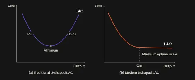
Reasons for the U-shaped LAC (traditional theory), panel (a):
- Law of returns to scale: the LAC is based on the long-run production function. In the early stage, increasing returns to scale lower the average cost, so LAC falls. Then constant returns give the minimum point. Finally, decreasing returns raise the average cost, so LAC rises. Together this produces a U shape.
- Economies of scale (falling part): as the firm expands, internal economies in production (specialized machinery, division of labour), marketing (bulk buying and selling), management (specialized departments), and transport and storage reduce cost per unit. External economies, such as cheaper finance and shared advertising, also lower costs.
- Diseconomies of scale (rising part): beyond the optimum size, managerial inefficiency, poor communication, labour inefficiency and lack of coordination appear. Rising input prices (external diseconomies) also push LAC upward.
- Planning curve: the LAC envelopes all the short-run average cost curves, and its lowest point shows the optimum plant size.
Reasons for the L-shaped LAC (modern theory), panel (b):
- Split of costs: modern theory divides total cost into production costs and managerial costs.
- Production costs keep falling: technical economies cause production costs to fall steeply at first and then slowly. Even after the minimum optimal scale (Qm), some economies continue, such as further decentralization, lower repair costs and producing some inputs in-house.
- Managerial costs rise only slowly: managerial costs first fall with better management techniques, and only at very large scales do they rise, and then only slowly.
- Net effect: the fall in production costs more than offsets the slight rise in managerial costs. So the LAC falls, reaches its minimum at Qm, and then stays roughly flat instead of rising. A rational producer keeps cutting costs through new ideas, technology and resources, so this L shape is considered more realistic. Beyond Qm, the LMC lies on or below the LAC.
The differences, with reasons, are as follows:
| Basis | U-shaped LAC | L-shaped LAC |
|---|---|---|
| Theory | Traditional (classical) theory | Modern theory |
| Shape after minimum | Rises, because diseconomies outweigh economies | Stays flat, because economies offset managerial costs |
| Main reason | Returns to scale (IRS, CRS, DRS); economies and diseconomies of scale | Continuing technical economies; managerial costs rise only slowly |
| Cost split | Not split | Production costs plus managerial costs |
| Realism | Less realistic | More realistic, supported by empirical studies |
Explore more questions
-
1.
Asked in 2082 (15 marks)
Critically analyze the Loanable Fund Theory of interest.
(ब्याजको ऋण योग्य कोषको सिद्धान्तको आलोचनात्मक विश्लेषण गर्नुहोस् ।)
-
2.
Long question Asked in 2082 (15 marks)
How does a cartel determine the price to maximize the joint profit? Evaluate the advantages and disadvantages of cartel for consumers and producers.
(संयुक्त नाफा अधिकतम गर्नका लागि कार्टेलले कसरी मूल्य निर्धारण गर्दछ ? उपभोक्ताहरू र उत्पादकहरूको लागि कार्टेलका फाइदाहरू र बेफाइदाहरू मूल्याङ्कन गर्नुहोस् ।)
-
3.
Long question Asked in 2082 (15 marks)
The production function of Langtang Cheese Pvt. Ltd. is \( Q = 4L + 11L^2 - L^3 \). Complete the following table.
(लाङटाङ चिज प्रा.लि.को उत्पादन फलन \( Q = 4L + 11L^2 - L^3 \) छ । दिइएको तालिका पूरा गर्नुहोस् ।)
No. of Labor Total Production Average Production Marginal Production 0 1 2 3 4 5 6 7 8 9 a) Analyze the three stages of the Law of Variable proportion for Langtang Cheese Pvt. Ltd. by using above data.
(माथिको तथ्याङ्क प्रयोग गरी लाङटाङ चिज प्रा.लि.का लागि परिवर्तनशील अनुपातको नियमका तीनवटा चरणहरुको विश्लेषण गर्नुहोस् ।)
b) Market price of cheese is Rs.1000 per kg. and the wage rate is Rs 34,000 per month. Using data of the second stage of the Law of Variable proportion, find the equilibrium level of labour and output of the cheese.
(चिजको बजार मूल्य प्रति केजी रु.१००० छ, र ज्याला दर प्रति महिना रु.३४००० छ । परिवर्तनशील अनुपातको नियमको दोस्रो चरणको तथ्याङ्क प्रयोगगरी, श्रम र चिजको उत्पादनको सन्तुलनस्तर पत्ता लगाउनुहोस् ।)
-
4.
Long question Asked in 2082 (10 marks)
Complete the following table. Graph total revenue, average revenue and marginal revenue curves. Explain the relation of total revenue and marginal revenue with price elasticity of demand.
(दिइएको तालिका पूरा गर्नुहोस् । कुलआय, औसतआय र सिमान्त आय वक्रहरूको ग्राफ बनाउनुहोस् । मागको मूल्यलोचसँग कुल आय र सिमान्त आयको सम्बन्ध व्याख्या गर्नुहोस् ।)
Quantity 0 10 20 30 40 50 60 70 Total revenue 0 60 100 120 120 100 60 0 Average revenue marginal revenue -
5.
Long question Asked in 2082 (10 marks)
Explain the consumer's equilibrium in cardinal approach. Price apple is Rs.20, price of banana is Rs. 10 and the consumer spends whole income Rs.110 on apple and banana. Find the consumer's equilibrium when the marginal utilities (MU) of apple and banana are as follows:
(संख्यात्मक उपयोगिता विश्लेषण विधिमा उपभोक्ता सन्तुलनको व्याख्या गर्नुहोस् । स्याउको मूल्य रु.२० छ, केराको मूल्य रु. १० छ र उपभोक्ताले आफ्नो सबै आम्दानी रु.११० स्याउ र केरामा खर्च गर्दछ । स्याउ र केराको सिमान्त उपयोगिताहरु निम्नानुसार भएको अवस्थामा उपभोक्ताको सन्तुलन पत्ता लगाउनुहोस् ।)
Units of consumption 1 2 3 4 5 6 7 MU of apple 800 700 600 500 400 300 200 MU of banana 500 450 400 350 300 250 200 -
6.
Asked in 2082 (10 marks)
Explain the degrees of elasticity of supply.
(पूर्तिलोचका श्रेणीहरुको व्याख्या गर्नुहोस् ।)
Question
Open in new tabCouldn't load this question. Open it instead.