Critically analyze the Marginal Productivity Theory of Wages.

A wage is the payment made to labour for its services in production. The marginal productivity theory of wages, developed by J.B. Say, J.B. Clark, A.C. Pigou and Alfred Marshall, states that the wage rate is determined by the marginal productivity of labour. A firm keeps hiring workers until the value of the marginal product of labour equals the marginal cost of labour (the wage rate):

VMPL = MCL (or MRPL = MCL)

The key terms are:

1. MPL (marginal productivity of labour) = ΔTP / ΔN: the extra output from one more worker.
2. VMPL (value of the marginal product) = MPL × price of the output: the money value of that extra output.
3. MCL (marginal cost of labour): the extra cost of hiring one more worker, which equals the wage rate under perfect competition.

The assumptions of the theory are:

4. Labour is the only variable factor, and all units of labour are homogeneous.
5. Perfect competition and perfect mobility of factors.
6. Full employment in the long run.
7. The law of diminishing returns applies to labour.
8. Perfect knowledge of the market wage rate for both workers and employers.

Explanation of the theory:

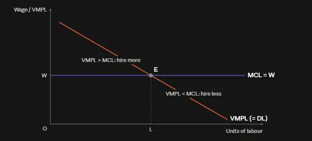
Demand for labour: as more workers are hired, MPL falls because of diminishing returns. With the output price constant, VMPL also falls, so the VMPL curve slopes downward. This curve is the firm’s demand curve for labour.

Supply of labour: under perfect competition, the firm can hire any number of workers at the market wage, so the supply (MCL) curve is a horizontal line at the wage rate.

Equilibrium: the firm is in equilibrium at E, where VMPL = MCL, and hires OL workers at wage OW. To the left of E, VMPL is greater than MCL, so hiring an extra worker adds more to revenue than to cost and the firm hires more. To the right of E, VMPL is less than MCL, so the firm hires fewer workers. For example, with a wage of Rs. 500, a firm hires 4 workers, because at that point VMPL = MCL = Rs. 500. Similarly, a tea estate in Ilam keeps hiring pickers until the value of the extra leaves picked just equals the daily wage.

Merits:

• The theory explains clearly why more productive workers, and workers in industries with high output prices, earn higher wages.
• It also explains why a firm’s demand curve for labour slopes downward.

Criticisms:

1. Unrealistic assumptions:
   a. Perfect competition, perfect knowledge and perfect mobility of labour do not exist in reality. Labour markets in Nepal, for example, have trade unions, monopsony employers and little mobility.
   b. All workers are not homogeneous; they differ in skill and efficiency.
   c. Full employment rarely exists, as unemployment is common.
2. Difficulty of measuring MPL: output is produced jointly by labour, capital and other factors, so it is very difficult to separate the marginal product of one worker, especially in services such as teaching or management.
3. One-sided theory and other practical problems:
   a. The theory explains only the demand side of labour (VMPL) and ignores the supply side, such as workers’ preferences, the cost of living and bargaining power.
   b. Under bilateral monopoly or collective bargaining, the wage is set by negotiation rather than by marginal productivity.
   c. Minimum wage laws and government policy also fix wages, regardless of VMPL.
   d. Under imperfect competition, workers are often paid less than their VMPL, which is called exploitation.
   e. It is a static, long-run theory and does not explain short-run wage changes or wage differentials caused by custom and discrimination.

The marginal productivity theory shows that a firm hires labour up to the point where VMPL equals the wage. It explains well why the demand for labour slopes downward and why productivity affects wages. However, because of its unrealistic assumptions and its neglect of the supply side and of bargaining, it is not a complete theory of wages.