This unit covers utility and consumer behaviour: cardinal and ordinal approaches, total, average and marginal utility, the law of diminishing marginal utility, the law of substitution (equi-marginal utility), and consumer’s and producer’s surplus, with numerical exercises.
Concept of utility and consumer behaviour
The person who purchases goods and services for their own consumption is known as a consumer. The study of the behaviour of an individual consumer or household is called consumer behaviour.
The power contained in goods and services to satisfy human wants is known as utility. The satisfaction that a consumer derives from the consumption of goods and services they buy is called their utility.
There are two approaches to the theory of consumer behaviour:
Cardinal utility
Cardinal utility is propounded by Alfred Marshall. When the consumer consumes goods and services and gets utility in numerical form like 1, 2, 3, 4, 5 and so on, it is called cardinal utility. It is measured in an imaginary unit known as a util.
Ordinal utility
The concept of ordinal utility was propounded by Edgeworth and Fisher in the early 20th century and later popularized by Pareto. It assumes that utility from goods and services cannot be measured in numbers, but satisfaction can be ranked in the order of 1st, 2nd, 3rd, and so on. A common assumption of both concepts is that the consumer is rational while consuming goods and services.
Total, average and marginal utility
Total utility (TU)
Total satisfaction derived from various units of consumption of goods and services is known as total utility. It is also the sum of marginal utilities that a consumer derives from continuous consumption of a commodity.
$$TU = \sum MU = MU_1 + MU_2 + \cdots + MU_n$$
Average utility (AU)
Average utility is per-unit utility of a commodity consumed. It is total utility divided by units of commodity consumed:
$$AU = \frac{TU}{Q}$$
Marginal utility (MU)
Additional utility derived from consumption of an additional unit of a commodity is known as marginal utility. It is also the ratio of change in total utility to change in quantity consumed:
$$MU = \frac{\Delta TU}{\Delta Q} = TU_n - TU_{n-1}$$
Derivation of TU, AU and MU
| Quantity consumed (Q) | MU | TU (= Σ MU) | AU (= TU/Q) |
|---|---|---|---|
| 1 | 10 | 10 | 10 |
| 2 | 8 | 18 | 9 |
| 3 | 6 | 24 | 8 |
| 4 | 4 | 28 | 7 |
| 5 | 2 | 30 | 6 |
| 6 | 0 | 30 | 5 |
| 7 | −2 | 28 | 4 |
Total utility initially increases and becomes maximum when MU is zero (at 6 units), then falls. Average utility falls as quantity consumed increases. After MU becomes zero, further consumption makes MU negative.
Relationship between TU and MU: when MU is positive, TU rises; when MU is zero, TU is maximum; when MU is negative, TU falls.
Law of diminishing marginal utility
The law of diminishing marginal utility was propounded by Herman Heinrich Gossen in 1854 (first law of Gossen). Credit for popularizing it scientifically goes to Alfred Marshall in Principles of Economics (1890).
The law states that when a rational consumer consumes more and more units of a commodity, marginal utility falls.
According to Alfred Marshall, “The additional benefit which a person derives from an increase of his stock of a thing diminishes with every increase in the stock that he already has.”
Assumptions
- Consumer should be rational.
- Price of the good should not change.
- Utility is measured in cardinal numbers.
- Marginal utility of money remains constant.
- The commodity should be divisible in nature.
Illustration
| Quantity consumed | Marginal utility |
|---|---|
| 1 | 10 |
| 2 | 8 |
| 3 | 6 |
| 4 | 4 |
| 5 | 2 |
| 6 | 0 |
| 7 | −2 |
When the consumer consumes the 1st unit, MU is 10. As units increase, MU falls. At the 6th unit MU is zero (full satisfaction), then becomes negative. Thus the table shows the law of diminishing marginal utility.
Exceptions / limitations
Rare and curious goods: goods hardly available and of high market value (old stamps, diamonds, old coins, rare paintings). Collectors may get more satisfaction from additional units, so MU may increase.
Dissimilar / heterogeneous goods: units must be homogeneous for the law. If later units are of superior quality, MU may increase.
Irrational / abnormal consumers: the law may not apply to misers, drunkards, gamblers, etc., where MU may rise.
Durable goods: cars, computers, machinery are generally indivisible; the law assumes divisible units.
Time gap: if there is a gap between consumption acts, MU may rise rather than fall.
Law of substitution (equi-marginal utility)
The law of substitution was propounded by H.H. Gossen in 1854 (second law of Gossen). It is also known as the law of equi-marginal utility or the law of maximum satisfaction. Alfred Marshall developed its present form.
Human wants are unlimited but means are limited. A consumer tries to get maximum satisfaction out of limited income by allocating income so that the last unit of money spent on each commodity yields equal marginal utility. A rational consumer substitutes one commodity for another until marginal utilities from the last units of all commodities become equal.
$$\frac{MU_x}{P_x} = \frac{MU_y}{P_y} = MU_m$$
Where \(MU_x\), \(MU_y\) are marginal utilities of X and Y; \(P_x\), \(P_y\) are prices; \(MU_m\) is marginal utility of money.
Assumptions
- Consumer should be rational.
- Income of consumer and prices of commodities are constant.
- Marginal utilities of different commodities differ.
- The law of diminishing marginal utility applies.
- Utility is measured in cardinal numbers.
Illustration
Suppose income is Rs. 5 and price per unit of each commodity is Rs. 1.
| Units | \(MU_x\) | \(MU_y\) |
|---|---|---|
| 1 | 20 | 16 |
| 2 | 16 | 12 |
| 3 | 12 | 8 |
| 4 | 8 | 4 |
| 5 | 4 | 0 |
Both MU schedules fall. The consumer reaches equilibrium where MU from both goods is equal (here at 12), using the limited income of Rs. 5 under the law of substitution.
Importance
- Importance to the consumer
- Importance to the producer
- Importance in exchange
- Importance to the government
- Importance in distribution
Exceptions / limitations
- Increase of marginal utility
- Custom and fashion
- Unlimited resources
- Indivisible goods
- Instability in price
Consumer’s surplus
The theory of consumer’s surplus was introduced by French engineer A.J. Dupuit (1844) and developed by Alfred Marshall. Marshall first called it “consumer’s rent,” later “consumer’s surplus.” K.E. Boulding called it “buyer’s surplus.”
According to Alfred Marshall, “Excess of the price which a consumer will be willing to pay rather than go without a thing over that which he actually does pay is the economic measure of this surplus satisfaction. It may be called the consumer’s surplus.”
Consumer’s surplus is the difference between expected (willingness-to-pay) price and actual price. Example: expected price Rs. 4500, actual price Rs. 4000 → surplus Rs. 500.
$$CS = EP - AP$$
Assumptions
- Utility can be measured in cardinal numbers.
- Marginal utility must be greater than price.
- Expected price must be greater than actual price.
- MU of money remains constant.
- Consumer should be rational.
| Units | Expected price (MU) | Actual price | Consumer’s surplus |
|---|---|---|---|
| 1 | 10 | 4 | 6 |
| 2 | 8 | 4 | 4 |
| 3 | 6 | 4 | 2 |
| 4 | 4 | 4 | 0 |
| Total | 28 | 16 | 12 |
The consumer buys up to where MU equals price. Total expected payment is Rs. 28; total actually paid is Rs. 16; total consumer’s surplus is Rs. 12.
Importance of consumer’s surplus
- Determine rate of tax
- Price determination
- Measurement of the benefit from international trade
- Distinction between value-in-use and value-in-exchange
- Measurement of economic development
Producer’s surplus
The concept of producer’s surplus was introduced by Alfred Marshall in Principles of Economics (1890). It is the excess of the price the producer receives over the lowest price at which the producer would be willing to sell.
Producer’s surplus = actual (market) price − minimum price willing to accept.
Example: willing to sell at Rs. 100, market price Rs. 150 → surplus Rs. 50.
Assumptions
- Rational producer
- Producer’s main motive is to earn profit
- Technology remains constant
- Actual market price is greater than minimum supply price
| Quantity sold | Actual (market) price | Minimum supply price | Producer’s surplus |
|---|---|---|---|
| 1 | 500 | 100 | 400 |
| 2 | 500 | 200 | 300 |
| 3 | 500 | 300 | 200 |
| 4 | 500 | 400 | 100 |
| 5 | 500 | 500 | 0 |
| Total | — | — | 1000 |
Total producer’s surplus is Rs. 1000.
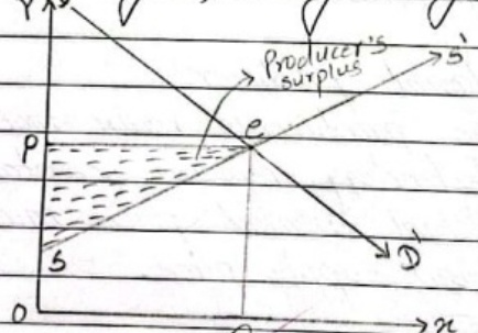
DD is demand and SS is supply. The minimum price the producer is willing to accept is along the supply curve; actual price received is OP. Total producer’s surplus is the shaded area between market price and the supply curve up to equilibrium quantity.
Numerical exercises
Exercise 1 — TU and MU schedule
| Units (Q) | Total utility (TU) | Marginal utility (MU) |
|---|---|---|
| 1 | 16 | 16 |
| 2 | 30 | 14 |
| 3 | 42 | 12 |
| 4 | 52 | 10 |
| 5 | 60 | 8 |
| 6 | 66 | 6 |
| 7 | 70 | 4 |
(MU for the 7th unit is \(70 - 66 = 4\).)
Exercise 2 — TU, MU and AU
| Q | TU | MU | AU |
|---|---|---|---|
| 1 | 1000 | 1000 | 1000 |
| 2 | 1800 | 800 | 900 |
| 3 | 2400 | 600 | 800 |
| 4 | 2800 | 400 | 700 |
| 5 | 3000 | 200 | 600 |
| 6 | 3000 | 0 | 500 |
| 7 | 2800 | −200 | 400 |
Exercise 3 — MU from a TU function
Given \(TU_x = 500x^3 + 50x^2 + 100x\), find \(MU_x\) and values at \(x = 10\).
$$MU_x = \frac{dTU_x}{dx} = 1500x^2 + 100x + 100$$
At \(x = 10\): \(MU_x = 151{,}100\); \(TU_x = 506{,}000\).
Exercise 4 — Equi-marginal allocation
Aarchi has Rs. 55 to spend on X and Y; price of each is Rs. 5 per unit.
| Q | \(MU_x\) | \(MU_y\) |
|---|---|---|
| 1 | 100 | 120 |
| 2 | 80 | 100 |
| 3 | 60 | 80 |
| 4 | 40 | 60 |
| 5 | 20 | 40 |
| 6 | 0 | 20 |
| 7 | −20 | 0 |
Total units affordable = \(55/5 = 11\). Maximum satisfaction is where MU from both goods is equal at 20: consume 5 units of X and 6 units of Y.
Exercise 5 — Equi-marginal (Rs. 5 income)
Income Rs. 5; price Rs. 1 each.
| Q | \(MU_x\) | \(MU_y\) |
|---|---|---|
| 1 | 10 | 12 |
| 2 | 8 | 10 |
| 3 | 6 | 8 |
| 4 | 4 | 6 |
| 5 | 2 | 4 |
| 6 | 0 | 2 |
| 7 | −2 | 0 |
Consume 2 units of X and 3 units of Y so that MU from both is 8.
Exercise 6 — Another TU function
Given \(TU_x = 20x^3 + 10x^2 + 5x\):
$$MU_x = 60x^2 + 20x + 5$$
At \(x = 4\): \(TU_x = 1460\); \(MU_x = 1045\).
Exercise 7 — Consumer’s surplus
| Units | Expected price | Actual price | Surplus |
|---|---|---|---|
| 1 | 1000 | 200 | 800 |
| 2 | 800 | 200 | 600 |
| 3 | 600 | 200 | 400 |
| 4 | 400 | 200 | 200 |
| 5 | 200 | 200 | 0 |
Total consumer’s surplus = \(800 + 600 + 400 + 200 + 0 = 2000\).
Exercise 8 — Producer’s surplus
| Units | Minimum price | Actual price | Surplus |
|---|---|---|---|
| 1 | 100 | 500 | 400 |
| 2 | 200 | 500 | 300 |
| 3 | 300 | 500 | 200 |
| 4 | 400 | 500 | 100 |
| 5 | 500 | 500 | 0 |
Total producer’s surplus = 1000.
If minimum price is Rs. 50 and market price is Rs. 250: producer’s surplus = \(250 - 50 = 200\).