This unit covers the concept of elasticity, price, income and cross elasticity of demand, factors that determine price elasticity, and the concept and types of elasticity of supply, with numerical exercises.
Concept of elasticity of demand
The term elasticity refers to the flexibility or change in position of something. In economics, elasticity is used to analyze the rate of change between price and demand, and between price and supply.
The law of demand tells that the quantity demanded for a commodity changes inversely with price. But it does not tell how much quantity demanded changes with the change in price. To identify the actual measure of change in price of a commodity and consequent quantity demanded, the concept of elasticity is used.
In brief, elasticity of demand measures the rate of change in quantity demanded as a result of the change in price. In other words, it is the measure of responsiveness of demand for a commodity to the change in any of its determinants.
The concept of elasticity of demand was first introduced by classical economists A.A. Cournot and J.S. Mill. Later, neo-classical economist Alfred Marshall developed it scientifically in his book Principles of Economics (1890).
According to Alfred Marshall, “The elasticity of demand in a market is great or small according as the amount demanded increases much or little for a given fall in price and diminishes much or little for a given rise in price.”
According to R.G. Lipsey, “Elasticity of demand may be defined as the ratio of the percentage change in the demand to the percentage change in the price.”
The major types of elasticity of demand are:
- Price elasticity of demand
- Income elasticity of demand
- Cross elasticity of demand
Price elasticity of demand
Price elasticity of demand is the ratio of the percentage change in quantity demanded to the percentage change in price of a commodity (other things remaining the same).
It is written as:
$$e_p = \frac{\text{Percentage change in quantity demanded}}{\text{Percentage change in price}}$$
Symbolically:
$$e_p = -\frac{\Delta Q}{\Delta P} \times \frac{P}{Q}$$
Where \(\Delta Q = Q_2 - Q_1\) (change in quantity), \(\Delta P = P_2 - P_1\) (change in price), \(P = P_1\) (initial price), and \(Q = Q_1\) (initial quantity). The negative sign is often used because price and quantity demanded move in opposite directions.
Types of price elasticity of demand
There are five types (degrees) of price elasticity of demand.
| Type | Value of \(e_p\) | Meaning |
|---|---|---|
| Perfectly elastic | \(e_p = \infty\) | Negligible price change → infinite change in quantity demanded |
| Perfectly inelastic | \(e_p = 0\) | Any price change → no change in quantity demanded |
| Unitary elastic | \(e_p = 1\) | % change in quantity = % change in price |
| Relatively elastic | \(e_p > 1\) | % change in quantity > % change in price |
| Relatively inelastic | \(e_p < 1\) | % change in quantity < % change in price |
Perfectly elastic demand (\(e_p = \infty\))
If the quantity demanded for a commodity increases infinitely with a very small (negligible) decrease in price, it is known as perfectly elastic demand. Such a situation is rarely found in the real world. It is written as \(e_p = \infty\).
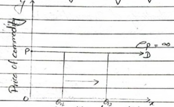
In the above figure, quantity demanded is measured along the X-axis and price along the Y-axis. PD is a demand curve which is a horizontal straight line parallel to the X-axis. It means that a negligible change in price causes an infinite change in quantity demanded.
Perfectly inelastic demand (\(e_p = 0\))
If there is no change in quantity demanded for a commodity with any change in its price, it is known as perfectly inelastic demand. Elasticity of demand is zero (\(e_p = 0\)). This case may be found in necessary commodities like salt, medicine, water, etc.
The demand curve is a vertical straight line parallel to the Y-axis. Price changes but quantity remains constant.
Unitary elastic demand (\(e_p = 1\))
If the percentage change in quantity demanded for a commodity is equal to the percentage change in its price, it is known as unitary elastic demand. This kind of price elasticity is largely imaginary and is rarely found in the real world.
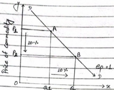
In the above figure, a fall in price results in the same percentage increase in quantity demanded.
Relatively elastic demand (\(e_p > 1\))
If the percentage change in quantity demanded for a commodity is greater than the percentage change in its price, it is known as relatively elastic demand. For example, if price changes by 5% and demand changes by 10%, demand is relatively elastic. This type can be found in demand for luxury commodities like car, computer, refrigerator, etc.
Relatively inelastic demand (\(e_p < 1\))
If the percentage change in quantity demanded for a commodity is less than the percentage change in its price, it is known as relatively inelastic demand. This type can be found in demand for basic/necessary commodities like rice, oil, cooking gas, vegetables, etc.
Income elasticity of demand
The percentage change in quantity demanded for a commodity due to the percentage change in the consumer’s income, price of commodities remaining constant, is known as income elasticity of demand.
$$e_y = \frac{\text{Percentage change in quantity demanded}}{\text{Percentage change in income}} = \frac{\Delta Q}{\Delta Y} \times \frac{Y}{Q}$$
Where \(e_y\) = income elasticity of demand, \(Q\) = quantity demanded, \(Y\) = income of the consumer, and \(\Delta\) denotes a small change. The value may be positive, negative, or zero depending on the nature of the commodity.
Types of income elasticity of demand
Zero income elasticity (\(e_y = 0\))
If quantity demanded is totally unresponsive to a change in the consumer’s income, demand has zero income elasticity. There is no relationship between the change in income and demand.
Positive income elasticity (\(e_y > 0\))
When quantity demanded increases with an increase in income and decreases with a decrease in income, income elasticity is positive (\(e_y > 0\)). Positive income elasticity is further divided as follows:
- Greater than unity (\(e_y > 1\)): percentage increase in quantity demanded is greater than the percentage increase in income (for example, income +5%, quantity +10%).
- Less than unity (\(e_y < 1\)): percentage increase in quantity demanded is less than the percentage increase in income (for example, income +10%, quantity +5%).
- Equal to unity (\(e_y = 1\)): percentage increase in quantity demanded equals the percentage increase in income.
Negative income elasticity (\(e_y < 0\))
When demand for a commodity decreases with an increase in the consumer’s income (and vice versa), income elasticity is negative (\(e_y < 0\)). This is typical of inferior goods.
Cross elasticity of demand
The percentage change in quantity demanded for a commodity due to the percentage change in the price of another (related) commodity is known as cross elasticity of demand.
$$e_{xy} = \frac{\text{Percentage change in quantity demanded of } x}{\text{Percentage change in price of } y} = \frac{\Delta Q_x}{\Delta P_y} \times \frac{P_y}{Q_x}$$
Where \(e_{xy}\) = cross elasticity of demand, \(Q_x\) = quantity demanded of X, \(P_y\) = price of Y, and \(\Delta\) denotes a small change.
Types of cross elasticity of demand
Positive cross elasticity (\(e_{xy} > 0\)): when two goods are close substitutes (for example, tea and coffee). If the price of tea rises, demand for coffee rises.
Negative cross elasticity (\(e_{xy} < 0\)): when two goods are complementary (for example, petrol and car). If the price of petrol rises, demand for cars falls.
Zero cross elasticity (\(e_{xy} = 0\)): when two goods are unrelated. A change in the price of Y does not affect demand for X.
Determinants of price elasticity of demand
Price elasticity of demand is determined by several factors.
Nature of the commodity
Demand for necessary commodities like salt is almost perfectly inelastic. Demand for basic commodities like rice, vegetables, and electricity tends to be relatively inelastic because a large price change brings only a small change in quantity demanded. Demand for luxury commodities like vehicles, washing machines, and refrigerators tends to be relatively elastic. Luxury wants can often be postponed when price rises.
Level of income
Rich consumers do not respond much to small price changes; their demand remains relatively inelastic. Poor consumers respond strongly to small price changes; even demand for basic commodities can be relatively elastic for them.
Existence of substitutes
Commodities with close substitutes have relatively elastic demand. For example, Coca-Cola and Pepsi are close substitutes. If the price of Coca-Cola rises while Pepsi’s price remains the same, quantity demanded of Pepsi increases. Goods without close substitutes (like salt) have less elastic demand.
Multiple uses of the commodity
Commodities that fulfill multiple purposes tend to be relatively elastic. For example, electricity can be used for lighting, heating, cooking, etc. At lower prices, more uses are adopted, so demand becomes more elastic.
Habit and custom
If a commodity is linked to habit or custom, demand is less elastic. For example, a rise in the price of cigarettes or wine may not reduce demand much. Likewise, during Dashain in Nepal, a rise in the price of goats may not reduce demand for mutton much.
Availability of time
If a consumer has sufficient time to buy, quantity demanded tends to be relatively elastic because cheaper alternatives can be found. If time is limited, demand tends to be relatively inelastic because the consumer must purchase quickly without much bargaining.
Elasticity of supply
The law of supply tells that quantity supplied of a commodity changes directly with price. But it does not tell how much quantity supplied changes with a change in price. The degree of change in supply due to a change in price is called elasticity of supply.
Elasticity of supply is the percentage change in quantity supplied divided by the percentage change in price:
$$e_s = \frac{\text{Percentage change in quantity supplied}}{\text{Percentage change in price}} = \frac{\Delta Q}{\Delta P} \times \frac{P}{Q}$$
Types of elasticity of supply
| Type | Value of \(e_s\) | Meaning |
|---|---|---|
| Perfectly elastic | \(e_s = \infty\) | At a given price, any quantity can be supplied; curve parallel to X-axis |
| Perfectly inelastic | \(e_s = 0\) | Quantity supplied fixed regardless of price; curve parallel to Y-axis |
| Unitary elastic | \(e_s = 1\) | % change in quantity supplied = % change in price |
| Relatively elastic | \(e_s > 1\) | % change in quantity supplied > % change in price |
| Relatively inelastic | \(e_s < 1\) | % change in quantity supplied < % change in price |
Perfectly elastic supply (\(e_s = \infty\))
If suppliers can supply any quantity at a given price, supply is perfectly elastic. The supply curve is a horizontal straight line parallel to the X-axis. This situation is largely imaginary.
Perfectly inelastic supply (\(e_s = 0\))
If quantity supplied remains constant whatever the price, supply is perfectly inelastic. The supply curve is a vertical straight line parallel to the Y-axis. Supply of land in a nation is an example.
Unitary elastic supply (\(e_s = 1\))
If the percentage change in quantity supplied equals the percentage change in price (for example, both change by 10%), supply is unitary elastic.
Relatively elastic supply (\(e_s > 1\))
If the percentage change in quantity supplied is greater than the percentage change in price (for example, supply +10% when price +5%), supply is relatively elastic.
Relatively inelastic supply (\(e_s < 1\))
If the percentage change in quantity supplied is less than the percentage change in price (for example, supply +5% when price +10%), supply is relatively inelastic.
Numerical exercises
Exercise 1 — Price elasticity of demand
Quantity demanded for X commodity is 100 units at price Rs. 10. When price decreases to Rs. 5, demand increases to 150 units. Find the price elasticity of demand.
Given: \(P_1 = 10\), \(Q_1 = 100\), \(P_2 = 5\), \(Q_2 = 150\).
$$e_p = -\frac{\Delta Q}{\Delta P} \times \frac{P}{Q} = -\frac{150-100}{5-10} \times \frac{10}{100} = -\frac{50}{-5} \times \frac{1}{10} = 1$$
Hence, demand is unitary elastic.
Exercise 2 — Price elasticity from a demand function
The demand function for a commodity is \(P = 75 - 2Q\). Calculate the price elasticity of demand at price Rs. 20.
Solution: At \(P = 20\), \(20 = 75 - 2Q \Rightarrow Q = 27.5\). Rearranging, \(Q = 37.5 - 0.5P\), so \(\frac{\Delta Q}{\Delta P} = -0.5\).
$$e_p = -\frac{\Delta Q}{\Delta P} \times \frac{P}{Q} = -(-0.5) \times \frac{20}{27.5} = 0.36 < 1$$
Hence, demand is relatively inelastic at this point.
Exercise 3 — Income elasticity
If demand for a commodity increases by 20% as a result of an increase in income by 10%, find the income elasticity of demand.
$$e_y = \frac{20\%}{10\%} = 2$$
Ashim’s demand for Coca-Cola was 10 bottles a month when earning Rs. 25,000. When income increases to Rs. 40,000, demand rises to 13 bottles. Calculate income elasticity.
$$\Delta Y = 15{,}000,\quad \Delta Q = 3,\quad e_y = \frac{\Delta Q}{\Delta Y} \times \frac{Y}{Q} = \frac{3}{15{,}000} \times \frac{25{,}000}{10} = 0.5$$
Exercise 4 — Cross elasticity
Initial price of Y = Rs. 1500; initial demand for X = 200 units. Subsequent price of Y = Rs. 1700; subsequent demand for X = 600 units. Find cross elasticity.
$$\Delta Q_x = 400,\quad \Delta P_y = 200,\quad e_{xy} = \frac{400}{200} \times \frac{1500}{200} = 15$$
Since \(e_{xy} > 0\), X and Y are substitutes.
Demand for A is 5000 units when price of B is Rs. 10,000. When price of B rises to Rs. 15,000, demand for A falls to 3000 units. Find cross elasticity.
$$e_{xy} = \frac{\Delta Q}{\Delta P} \times \frac{P}{Q} = \frac{-2000}{5000} \times \frac{10{,}000}{5000} = -0.08$$
Since \(e_{xy} < 0\), A and B are complementary (not substitutes).
Exercise 5 — Elasticity of supply
Quantity supplied is 50,000 units at price Rs. 5000. When price falls to Rs. 4000, supply falls to 30,000 units. Find elasticity of supply.
$$\Delta Q = -20{,}000,\quad \Delta P = -1000,\quad e_s = \frac{\Delta Q}{\Delta P} \times \frac{P}{Q} = \frac{-20{,}000}{-1000} \times \frac{5000}{50{,}000} = 2$$
Exercise 6 — Price elasticity (computer)
When price of a computer increases from Rs. 40,000 to Rs. 44,000, quantity demanded falls from 1000 to 870 units. Find price elasticity of demand.
$$e_p = -\frac{870-1000}{44{,}000-40{,}000} \times \frac{40{,}000}{1000} = 1.3$$
Hence, demand is relatively elastic.
Exercise 7 — Point elasticities from a schedule
| Point | Price (Rs.) | Quantity demanded |
|---|---|---|
| A | 10 | 115 |
| B | 25 | 95 |
| C | 35 | 85 |
| D | 45 | 45 |
| E | 65 | 25 |
| F | 95 | 15 |
From B to C:
$$e_p = -\frac{85-95}{35-25} \times \frac{25}{95} = 0.26 < 1 \quad \text{(inelastic)}$$
From E to D (price falls from 65 to 45; quantity rises from 25 to 45):
$$e_p = -\frac{45-25}{45-65} \times \frac{65}{25} = 2.6 > 1 \quad \text{(elastic)}$$
Exercise 8 — Another schedule
| Point | Price (Rs.) | Quantity demanded |
|---|---|---|
| A | 105 | 165 |
| B | 91 | 175 |
| C | 89 | 185 |
| D | 75 | 200 |
| E | 25 | 300 |
| F | 5 | 560 |
From A to B:
$$e_p = -\frac{175-165}{91-105} \times \frac{105}{165} = 0.45 < 1 \quad \text{(inelastic)}$$
From F to C:
$$e_p = -\frac{185-560}{89-5} \times \frac{5}{560} \approx 0.04 < 1 \quad \text{(inelastic)}$$