This unit covers the market economy, demand and supply (meaning, laws, determinants, movement and shift), and how their interaction determines market equilibrium, with numerical exercises.
Market Economy
The theoretical basis for market economies was developed by classical economists such as Adam Smith, David Ricardo and Jean - Baptiste Say in the late 19th and early 20th centuries. These classically liberal free market advocates believed that protectionism and government intervention tended to lead to economic inefficiencies that actually made people worse off. A market economy is an economic system in which economic decisions and the pricing of goods and services are guided solely by the aggregate interactions of a country's individual citizens and businesses. There is little government intervention or central planning. This is the opposite of a centrally planned economy, in which government decisions drive most aspects of a country's economic activity. Market economies work on the assumption that forces such as supply and demand are the best determinants of aggregate well being
Features of the Market Economy
Supply and demand: the larger the available supply of goods or services relative to demand, the lower the price that can be charged; if demand is high and supply is low, price rises.
Competition: firms monitor pricing relative to rivals. More competition means closer attention to price and quality.
Profit motive: business owners aim to earn revenue above expenses by attracting customers at prices that yield profit.
Less government intervention: prices and allocation are set mainly by market conditions; government’s role is largely to help keep markets stable rather than dictate daily economic policy.
Perfect competition (ideal): rivalry among firms shapes the cost of goods and services as sellers seek profit while outperforming competitors.
Consumer freedom: buyers may choose which firms to deal with; they are not restricted to a single seller.
Demand
The amount of a particular economic good or service that a consumer or group of consumers will want to purchase at a given price is known as demand. The demand curve is usually downward sloping since consumers will want to buy more as price decreases. Along with supply, demand is one of the two key determinants of market price.
According to Milton H. Spencer, “Demand is the quantity that will be purchased of a particular commodity at various prices, at a given time and place.”
Meaning of Demand
In ordinary language, demand means a desire or want. In economics, demand is effective desire backed by ability to pay and willingness to pay at a particular time. Mere desire is not demand — for example, a poor person’s wish for an expensive car is only desire without ability to pay.
Requirements of demand:
- Desire for goods and services
- Willingness to pay
- Ability to pay
Difference between desire and demand:
| Desire | Demand |
|---|---|
| A human want or wish | Effective desire backed by ability and willingness to pay |
| Has no economic meaning by itself | Has economic meaning |
| Does not require purchasing power | Needs resources (ability to pay) |
| A poor person wanting a big house in Kathmandu — desire only | A billionaire wanting the same house — may be demand |
Demand Equation
When other determinants are constant, demand depends upon price. \( D = a - bp \)
D = Demand
a, b = Constant
P = Price
Types of Demand
Demand can be broadly classified into different types, which are explained as follows
Direct demand
The demand for an ultimate object is called direct demand. In other words, direct demand refers to the demand for a commodity that is directly consumed to satisfy human wants. For example, demand for bread, butter, fruits, etc. Direct demand for a commodity can be further classified into price demand, income demand, and cross demand
Price demand
Price demand refers to the various quantities of a commodity or services that a consumer would purchase at a given time period in a market at various prices. It expresses the relationship between price and quantity demanded. There would be higher demand at a lower price and lower demand at a higher price, other things, remaining the same. Consumer's income, his tastes and preferences price of related goods, etc. are the other things
Income demand
Income demand expresses the relationship between income and demand for a commodity. It refers to the various quantities of goods and services, which would be purchased by a consumer at various levels of income in a given period of time, other things being equal. Other things are the prices of the related goods, taste, and preferences of the consumer, price of the same good, etc. The demand for normal goods increases with the rise in income and vice-versa. But in the case of inferior goods, there is an inverse relationship between income and demand. In such a case, as income increases, demand decreases and vice-versa
Cross demand
Cross demand expresses the relationship between the demand for one good, say X, and the price of the related good, say Y. It refers to the various quantities of a good, which will be purchased with reference to the change in the price of other related goods. There are two types of related goods: substitute and complementary
- Substitute goods: Those goods are substitute goods, which are used in place of each other, for example, tea and coffee. If the price of tea increases, the demand for coffee will rise, and vice-versa, the price of coffee remains the same
- Complementary goods: Those goods are complementary goods, which are jointly used to satisfy a want, for example, pen and ink In such case, the rise in the price of a pen will bring a fall in the demand for ink. Conversely, a fall in the price of pens will increase the demand for ink
Indirect or derived demand
The demand for factors of production, which go to make the final product is called indirect or derived demand because they help in the production of a commodity, which is directly demanded by the consumer in the market. For example, the demand for brick, cement, iron, wood, labor, etc. to construct a building, is a derived demand
Joint demand
When several things are demanded for a joint purpose, it is a case of joint demand. In other words, the demand for complementary goods is joint demand because complementary goods are demanded jointly to satisfy a want. For example, the demand for cars and petrol, pen and ink, etc
Composite demand
When a good is demanded for several uses, it is called composite demand. For example, the demand for electricity is composite demand because it has several uses like heating, cooling, lighting, cooking, etc
Competitive demand
This type of demand exists when goods are close substitutes for each other. Ceteris paribus, when the price of NTC services rises, people will shift towards Ncell services. The demand for NTC and Ncell mobile is called competitive demand
Determinants of Demand
Demand for a commodity depends upon many factors. Factors determining the demand for a commodity are known as determinants of demand. The important determinants or factors affecting the demand are as follows
- Price of the commodity: The most important determinant of demand is the price of the same commodity. When the price of a commodity falls, its quantity demanded will increase and vice-versa. It means that there is an inverse relationship between the price and quantity demand for the commodity
- Income of the consumer: Demand for a commodity change when the income of the consumer changes. In the case of normal goods, when the income of the consumer rises, the demand also increases and vice versa. But, in the case of inferior goods, the demand for the commodity decreases with the rise in income and vice-versa. It means that there is a positive relationship between income and demand for normal goods and an inverse relationship between income and demand for inferior goods. For example, branded clothes kept to sell in shopping complexes are normal goods whereas low-quality clothes kept in streets to sell are inferior goods
- Prices of the related goods: The demand for a commodity is also determined by the change in the prices of related goods. There are two types of related goods, which are as follows
Substitute goods: Those goods are substitute goods, in which one can be used in absence of another. In the case of these goods, if the price of one rises, the demand for another rises and vice-versa. For example, tea and coffee are substitute goods. If the price of tea increases, assuming the price of coffee is constant, the demand for coffee will increase and vice-versa
Complementary goods: Those goods are complementary goods, which are jointly used to satisfy a particular want. In the case of these goods, if there is a rise in the price of one good, assuming the price of a related good constant, the demand for other goods will fall and vice-versa. For example, pen and ink. If the price of a pen rises, the demand for ink will fall and vice versa
- Taste and preference of the consumer: Demand also depends on the taste and preference of the consumer. The change in consumer's tastes and preferences causes a change in demand for goods. If the taste and preference of a commodity are in favor of the consumer, the demand for that commodity will increase and vice-versa
- Advertisement: There is a great impact of advertisement. Goods, which are widely advertised, become popular and consumers are attracted to those goods. People can also take more information about various goods from the advertisement. As a result, the demand for those goods increases
- Income distribution: The distribution of income in society also affects the demand for goods. If the distribution of income is more equal, then the propensity to consume of the society will be relatively high. As a result, demand for goods increases. If the distribution of income is more unequal, the propensity to consume will be relatively low. As a result, demand for goods decreases. If income distribution is in favor of the rich, demand will be low. If income distribution is in the favor of the poor, demand will be high
- Size and composition of population: The size of the population also affects the demand for goods and services. When the size of the population increases, the demand for necessaries of life also increases and vice versa. The composition of population means the proportion of young, old and children as well as the ratio of men to women. The composition of the population also affects the composition of demand. For example, if the population of elderly people increases, the demand for medicine will increase
- Consumer's expectation: If a consumer expects a rise in the price of a commodity in the near future, he will demand more quantities of that commodity at the present time so that he should not have to pay a higher price in the future. Similarly, if the consumer expects he will have a good income in the future, he will spend the greater part of his income at present time. As a result, his present demand for goods will increase
- The availability of credit: Nowadays, the demand for many durable consumer goods like cars, furniture, television, and other types of household equipment depends very much on the provision of credit facilities. Such credit facilities are provided by the banking sector on a monthly installment basis. If there is any change in terms of this type of finance, there will be a marked effect on demand for such types of goods
- Climate and weather: The demand for goods is also affected by the climate and weather. In the winter season, the demand for warm clothes will rise and during the summer, the demand for cotton clothes will rise. Similarly, there will be high demand for umbrellas and rain coats during the rainy season
Demand Function
The functional or mathematical relationship between the quantity demand for goods and the factor determinants of demand is known as the demand function
The mathematical relationship between quantity demand for goods and factor determinants of quantity demand or demand function can be expressed in the algebraic form
It is presented by:
D = f(P_{x}, T, Tech...)
Where
y = Income
= Taste and Preference
Tech = Technology
Law of Demand
The law of demand states that when the price of a commodity rises, quantity demanded falls, and vice versa, other things remaining the same — an inverse relationship between price and quantity demanded.
Symbolically,
\( \uparrow D = f(P) \downarrow \)
and
Vice-Versa
Where,
D = Quantity demanded
f = function
P = Price
The law of demand is based on some pre-conditions which are known as assumptions of law of demand which are as follows
- No change in income of consumer
- No change in consumers' taste and preference
- No change in season
- No change in technology
- No change in size of population
Based on the assumptions above, the law of demand is explained by the following schedule.
Table: Law of Demand Schedule
| Price of commodity (Rs per unit) | Quantity demanded (kg) |
|---|---|
| 50 | 10 |
| 40 | 20 |
| 30 | 30 |
| 20 | 40 |
| 10 | 50 |
It is presented by following figure
| Point | x | price |
|---|---|---|
| A | 25 | 50 |
| B | 35 | 35 |
| C | 50 | 25 |
| D | 50 | 10 |
Quantity Demanded
(in kg)
fig: 2.1
In the above fig 2.1, x-axis measures quantity demanded and y-axis measures price of commodity. When price is Rs 50 quantity demanded is 10 kg. When price falls to Rs 40, 30, 20, and 10 then quantity demanded rises to 20 kg, 30, 40 and 50 kg respectively. When we join the points A, B, C, D and E then we get demand from DD'. If is downward sloping curve. It shows inverse relationship between price of commodity and quantity demanded. Therefore above figure shows the law of demand
Causes of Demand Curve Sloping Downwards
(1) Law of diminishing marginal utility: The consumer in order to restore the new equilibrium between price and utility buys more of it so that the marginal utility falls with the rise in the amount demanded. So long the price of a commodity falls, the consumer will go on buying more amount of it so as to reduce the marginal utility and make it equal with new price. Thus, the shape and slope of a demand curve is derived from the slope of marginal utility curve
(2) Income effect: As the price of a commodity falls, the consumer has to buy the same amount of the commodity at less amount of money. After buying his required quantity he is left with some amount of money. This constitutes rise in his real income. This rise in real income is known as income effect. This increase in real income induces the consumer to buy more of that commodity. Thus income effect is one of the reasons why a consumer buys more at falling prices
(3) Substitution effect: When the price of a commodity falls, it becomes relatively cheaper than other commodities. The consumer substitutes the commodity whose price has fallen for other commodities which becomes relatively dearer. For example, with the fall in price of tea, coffees, Price being constant, tea will be substituted for coffee. Therefore the demand for tea will go up
(4) New consumers: When the price of a commodity falls many other consumers who were deprived of that commodity at the previous price become able to buy it now as the price comes within their reach. For example, the units of color TV increases with a remarkable fall in price of it. The opposite will happen with a rise in prices
(5) Multiple use of commodity: There are some commodities which have multiple uses. Their uses depend upon their respective, prices. When their prices rise they are used only for certain selected purposes. That is why their demand goes down.For example electricity can be put to different uses like heating, lighting, cooling, cooking etc. If its price falls people use it for other uses other than that. A rise in price of electricity will force the consumer to minimize its use. Thus with a fall and rise in price of electricity its demand rises and falls accordingly
Demand Schedule, Demand Curve and Demand Equation
A demand schedule is a list of prices and demand. It explains the relationship between two variables, price, and quantity. it can be presented as follows: Price per kg Quantity Demanded Rs. 10 10 kg Rs. 8 20 kg Rs. 6 30 kg Rs. 4 40 kg Rs. 2 50 kg The above demand schedule shows a negative relationship between price and quantity demanded a commodity. Initially, when the price of a good is Rs.10 per kg, the quantity demanded by the consumer is 10 kg. As the price decrease from Rs.10 per kg to Rs.8 per kg and then to Rs.6 per kg, quantity demanded by the consumer increases from 10 kg to 20 kg and then to 30 kg respectively and so on
Demand Curve
The geometrical/ graphical representation of the demand schedule is a demand curve. it can be presented as follows: In the above figure, price and quantity demanded are measured along the y-axis and x-axis respectively. By plotting various combinations of price and quantity demanded, we get a demand curve DD1 derived from points A, B, C, D, and E
Demand Equation / Demand Function
Demand is also a functional concept. So, it can be expressed algebraically in the form of an equation or function. There are two types of the demand function, which are as follows
a) Simple demand function: The demand function showing simple relation is expressed in functional form as;
QD = 𝑓(p)
Where, QD = Quantity demanded and P = price
The above equation means that demand depends upon price
b) Multiple demand function: Multiple demand function refers to the functional relationship between demand and all the factors affecting demand. It is expressed as
QDx = 𝑓 (Px, Pr, Y, T, E, Py)
Where, QDx = Quantity Demanded for Commodity X; Px = Price of the given Commodity X; Pr = Prices of Related Goods; Y = Income of the Consumer; T = Tastes and Preferences; E = Expectation of Change in Price in future; Py = price of commodity Y The above equation states that demand for commodity X will depend on the above-listed variables
Exceptions / Limitations of the Law of Demand
- Violation of law of Demand
- Make failure law of Demand
\( \uparrow\overline{D}=f(P)\uparrow \)
\( \downarrow\overline{D}=f(P)\downarrow \)
There are several limitations or exceptions of the law of demand:
- Inferior and Lumurious goods
- Interior and numerous goods
To the case of demont for luxurious and inferior goods, there is a positive relationship between price and quantity demanded. A rise in the price of an interior good (low quantity goods) causes to buy more goods. Because the wages earners substitute on the diet only of low quality bread, when its price rises, they have to spend more money for a given quantity of bread. So to maintain their intake of food, they buy more bread at higher price
Similarly, some rich peoples try to measure the utility of goods and services by their corresponding price level. If the price of the luxurious goods falls, they become inferior to rich consumers. As a result, quantity demanded for those goods decrease despite the fall in price level
- Price Expectation
- Rare Collection
- In the case of rare collection like;
Stamp Collection
Old coin collection
Signature
Yarsagumba, etc
the people ready to buy more goods even
if the price is high. So, in rare collection,
the law of demand is not applied
- Out of fashion
- If the commodity goes out of fashion, consumers do not purchase more even if the price falls
As for example, the demand for typical Nepali clothes Daura Sunual and Gunyan Choli has sharply decreased even if the relative price is low. If is because their use has gone out of fashion
- Change in income of consumers
There is a positive relationship between quantity
demanded for a good and income of the consumer
Hence, when income of the consumer increases, the
demand for goods also increases, even if the price
of goods goes up
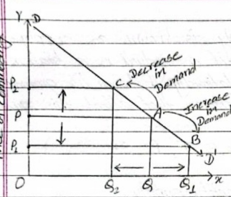
Movement along a Demand Curve
- If is occurred due to change in price and non-price factors remain constant here. Following are non-price factors
Price of related goods
Income of consumers
Taste and Preferences
Size of population
Technology
Season etc
It is presented by following diagram
| Variable | Q₁ | Q₂ | Q₃ | Q₄ |
|---|---|---|---|---|
| Y | 100 | 100 | 100 | 100 |
| D | 100 | 100 | 100 | 100 |
| C | 100 | 100 | 100 | 100 |
| A | 100 | 100 | 100 | 100 |
| B | 100 | 100 | 100 | 100 |
| D' | 100 | 100 | 100 | 100 |
| Demand | 100 | 100 | 100 | 100 |
Quantity Demanded
fig: 2.1
To the given figure 2.1, quantity demanded for a goods is measured along the OX-axis and price of the goods is measured along the OY-axis DD' is demand curve. When price of a good is OP, the demand is OO. When price of goods decreases from OP to OP, the quantity demanded for the goods increases from OO to OO, due to this movement occurs from point A to B, it is called extension of demand. Similarly, if price increases from OP to OP, the quantity is depended for a good decreases from OO to OO, due to this the movement occurs from point A to C, it is called contraction of demand
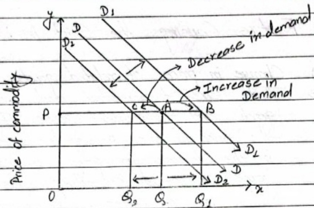
Shift in Demand Curve
- TE is occurred due to change in non-price factor like;
But price remains constant here
It is presented by following diagram
Price of commodity
Quantity demanded
fig: 2.2
In the figure 2.2. quantity demanded for a goods is measured along OX-axis and price of the goods is measured along the OY-axis. DD is initial demand curve. In this demand curve, QQ quantity of goods is demanded by consumer at price OP. Let is assume, the quantity demanded for a good increases from QQ to QQ due to the change in non-price determinants of demand like fashion, season, technology etc., remaining the price constant at OP, the demand curve DD shifts to right from the point A to B as new demand curve \( D_{1}D_{2} \) it is called increase demand. Similarly, when demand decreases from QQ to Q2 price remaining constant, the initial demand curve DD shifts to the left from point A to C as new demand curve \( D_{2}D_{3} \), it is called decrease in demand
Difference between Movement and Shift in Demand Curve
| Movement along the demand curve | Shift in demand curve |
|---|---|
| Movement along demand curve can be defined as graphical representation of change in demand for a commodity brought by change in its own price other things remaining constant | A demand curve changes its position either upward or downward from its initial point due to the change in quantity demanded for a good because of change in non-price factors determinants of demand like fashion, season, price of related goods etc. price remains constant it is known as Shift in demand curve |
| Movement along a demand curve occurred due to change in price factors but non-price factors remain constant here | Shift in Demand curve is occurred due to change in non-price factors but price remains constant here |
| A movement along the curve can be traced up and down along the same curve | The shift in the demand curve occurs when the demand curve changes |
| Movement along a demand curve result in expansion or contraction in demand | There are upward shifts and downward shifts in the demand curve |
| Movement along a demand curve is also termed as ‘change in quantity demanded.’ | A shift in the demand curve is also termed as a ‘change in demand.’ |
| Movement along a demand curve does not affect the equilibrium | The shift in the demand curve changes the equilibrium |
Quantity demanded
| Point | Price / Demand | Price / Demand |
|---|---|---|
| A | 30 | 30 |
| B | 50 | 50 |
| C | 25 | 25 |
| D | 50 | 50 |
| D₁ | 100 | 100 |
| D₂ | 100 | 100 |
| D₃ | 100 | 100 |
Quantity demanded
Individual and Market Demand Curves
Individual demand curve
The individual demand curve represents the quantity of a good that a consumer will buy at a given price, holding all else constant. For example, consumer A might buy 2 orange at RS. 10 each, 4 oranges at Rs. 7 each, and 6 at Rs 4 each, while consumer B might buy 3 oranges at Rs. 10, 6 oranges at Rs 7, and 7 at Rs 4 . When charted on a graph with price on the vertical axis and quantity purchased on the horizontal axis, these points form the individual demand curves for consumers A and B
Market demand curve
The market demand curve is the sum of all the individual demand curves in the market. If the entire market consisted of only the two consumers mentioned above, the total demand for oranges at a price of Rs 10 would be 5 oranges, because A would buy 2 and B would buy 3 oranges. At a price Rs 7, the market demand would be ten oranges, summing A's 4 oranges and B's 6. For a single good, adding all the individual demand curves of the millions of consumers in the market makes the total market demand curve
Factors Causing Shift in Demand Curve
| Factor | Rightward Shift | Leftward Shift |
|---|---|---|
| Change in the income of the consumer | Increase in income in case of normal goods but a decrease in income in case of inferior goods | Decrease in income in case of normal goods but increase in income in case of inferior goods |
| Change in price of related goods | A rise in the price of substitute goods but fall in the price of complementary goods | Fall in price of substitute goods but a rise in the price of complementary goods |
| Change in taste and preference | Favorable changes in taste and preference | Unfavorable change in taste and preference |
| Change in advertisement | Rise in advertisement expenditure | Fall in advertisement expenditure |
| Change in size of population | Increase in size of the population | Decrease in size of the population |
| Change in income distribution | More equal distribution of income | More unequal distribution of income |
| Price expectations | The expectation of a rise in the price for shortage or increase in future income | The expectation of fall in price or fall in future income |
| Availability of credit | More availability of credit provision | No or less availability of credit provision |
Supply
Meaning of Supply
Supply is the amount of something that firms, consumers, laborers, providers of financial assets, or other economic agents are willing to provide to the marketplace. In the goods market, supply is the amount of a product per unit of time that producers are willing to sell at various given prices when all other factors are held constant. In the labor market, the supply of labor is the amount of time per week, month, or year that individuals are willing to spend working, as a function of the wage rate. In the financial markets, the money supply is the amount of highly liquid assets available in the money market, which is either determined or influenced by a country's monetary authority
According to R. G. Lipsey, "The amount of a commodity that firms are able and willing to offer for sale is called the quantity supplied of that commodity."
Supply Function
The functional or mathematical relationship between the quantity supplied and the factor determinants of supply is known as the supply function. The supply function of a product is a statement of the mathematical relationship between the quantity supplied and the factors that affect this quantity
\( Q_{S}=f(P,P_{F},S,T,P_{e},S_{e}---) \)
where,
Qs = Quantity supply
f = function
P = Price
P = Price of factor of Production \( (R, W, T, P) \)
S = Season
T = Technology
Equation of Supply
If other factors are constant supply is the function of price. Its equation is
\( S = a + bp \)
$$ \begin{array}{c} S=\text{Supply}\\ a,b=\text{Constant}\\ P=\text{Price} \end{array} $$
Law of Supply
The law of supply is the microeconomic law that states that all other factors being equal, as the price of a good or service increases, the number of goods or services that suppliers offer will increase, and vice versa. The law of supply says that as the price of an item goes up, suppliers will attempt to maximize their profits by increasing the quantity offered for sale
There is positive relationship between quantity supply of a commodity and its price, other things remain constant. It means, the supply of commodity increases with the increase in price and vice versa. This tendency is called law of supply. When the price of a commodity rises, there is an increase in profit. Due to this the firms are induced to produce and sell more quantity in higher price. Therefore there is positive relationship between price of commodity and quantity supply
Symbolically,
$$ \uparrow S = f(P)\uparrow $$
Vice-Versa
Assumptions of Law of Supply
- Nature of Goods. If the goods are perishable in nature and the seller cannot wait for the rise in price. Seller may have to offer all of his goods at the current market price because he may not take risk of getting his commodity perished.
- Government Policies. The government may enforce the firms and producers to offer products at the prevailing market price. In such a situation producer may not be able to wait for the rise in price.
- Alternative Products. If a number of alternative products are available in the market and customers tend to buy those products to fulfill their needs, the producer will have to shift to transform his resources to the production of those products.
- Squeeze in Profit. Production costs like raw materials, labor costs, overhead costs, and selling and administration may increase along with the increase in price. Such situations may not allow the producer to offer his products at a particular increased price.
- No change in season.
- No change in state of technology.
- No change in price of factors of production.
Supply Schedule (Law of Supply)
The concept of law of supply can be explained with the help of a supply schedule and a supply curve
| Price per kg (Rs) | Quantity supplied |
|---|---|
| 10 | 50 kg |
| 8 | 40 kg |
| 6 | 30 kg |
| 4 | 20 kg |
| 2 | 10 kg |
In the above schedule, we can observe that when the price was Rs 10 per kg, quantity supplied was 50 kg. When the price declined to Rs 8 and Rs 6, the quantity supplied also decreased to 40 kg and 30 kg respectively and so on. This shows that, as price decreases, quantity supplied decreases and vice versa
Supply Curve (Law of Supply)
We can present the above schedule in a graph. The figure shows the combinations of price and quantity supplied as presented in the schedule above. When the combination points are joined together, we get an upward sloping curve (SS) known as the supply curve. It shows the positive relationship between price and quantity supplied
Exceptions / Limitations of the Law of Supply
- Expectations of a fall in price: If the firms anticipate that the price of the product will fall further in future, in order to clear their stocks they may dispose it off at a price that is even lower than the current market price
- Auction sale: Auction sale means selling of a product at competitively higher price making competition among many buyers. The law of supply does not hold good in case of auction sale. An auction sale may be made when a seller is badly in need of money. He may sell his goods at the price offered by the higher bidder. But the price offered may be higher or lower in comparison to the expected price. If the seller is in need of hard cash, he may sell his product at a price which may even be below the market price
- Clearance sale: If the firms want to shut down or close down their business, they may sell their products at a price below their average cost of production
- Seller's expectation: When a seller expects that there will be further fall in price of a commodity in future, he will try to sell more quantity even if the price is lower. Similarly, if he expects that there will be further rise in price of a commodity in future, he will not sell any more quantity even if the price is higher. Therefore, the law of supply does not exist true in case of price expectation of sellers
- Fear of being out of fashion: If there is probability of change in fashion of a commodity very soon, the seller will try to sell more quantity of the commodity even if price is lower. It is also opposite of the norms of law of supply
- Perishable goods: The law of supply does not apply in the case of perishable goods. Perishable goods are those goods which have short life span i.e. they should be consumed within certain time. Therefore the producer reduces price and sells more quantity in market
- Agricultural output: In agricultural production, natural and seasonal factors play a dominant role. Due to the influence of these constraints supply may not be responsive to price changes
- The backward sloping supply curve of labor: The rise in the price of a good or service sometimes leads to a fall in its supply. The best example is the supply of labor. A higher wage rate enables the worker to maintain his existing material standard of living with less work, and he may prefer extra leisure to more wages
Determinants of Supply
Those factors which change the quantity supplied of a commodity are known as determinants of supply. There are various factors that bring changes in quantity supply of a commodity. Some important factors that determine quantity supply are discussed as follows:
Price of the commodity (own price)
The price of the commodity is the most important determinant of supply. There is a direct relationship between the price of the commodity and its quantity supplied, other things remaining the same. It means that at the higher price, producers or sellers offer more quantity of a commodity for sale, and at a lower price, producers or sellers offer less quantity of the commodity for sale. The supply of a commodity increases with the increase in price and vice-versa. This tendency is called law of supply. When the price of a commodity increases, there is an increase in profit. This induces firms to produce and sell more quantity at higher price
Price of factors of production
Quantity supply of a commodity is highly affected by the price of factor of production. When price of factors of production increases, price of goods remains constant, the firm cannot supply the quantity of goods as before change in price of factors of production. Hence, when factor price increases the supply will decrease and vice-versa. With the rise in the price of factors of production, the cost of production also rises, which results in a decrease in supply and vice versa
Price of other goods
The supply of a particular commodity is inversely related to the price of other commodities. For example, a rise in the price of rice will fall the supply of wheat. This is due to the fact that a rise in the price of rice will encourage producers to produce more rice
Season
Season also affects the quantity supply of a commodity. Some goods are demanded in a specific season. So, the supplier supplies the product only when it is demanded in the market. For example, the supply of ice cream increases in the summer season and supply of woolen cloths is increased in the winter season. Similarly, the supply of different fruits is increased in the harvesting season because production of these fruits and vegetables increase in the particular season. Hence, the season affects the quantity supply of a product
Technological change
If there is technological progress in production process, more quantity of quality goods can be produced at lower cost which helps to increase the quantity supply of that commodity in the market. Similarly, if the state of technology becomes old and inefficient in the production the producer will unable to supply more quantity and supply will decrease. Improvement in technology has a positive effect on the supply of the commodity. It reduces the per-unit cost of production. Consequently, the profit of the business firm will increase. In order to earn more profit, firms increase the supply of the commodity
Seller's expectation
If seller expects the price of goods will decrease in near future, he/she increases the quantity of supply. On the contrary, if he expects the price of goods will increase in near future, he decreases the supply. Similarly, if seller has fear of out of fashion of product produced by him, he increases the supply at present. Hence, seller's expectation also affects the quantity supply of a commodity. If the producers expect a rise in the price of the commodity in the near future, the current supply of the commodity decreases. On the other hand, if they expect a fall in the price, the current supply increases
Goal of the firm
If the goal of the firm is to maximize profit, less quantity of the commodity will be offered for sale at a high price. On the other hand, if the goal of the firm is to maximize sales or revenue or maximize output or employment, more will be supplied even at the lower price
Government policy
Taxation and subsidy policies of the government also affect the market supply of the commodity. An increase in taxation tends to reduce the supply, while subsidies tend to induce a greater supply of the commodity
The number of firms
The market supply of a commodity also depends upon the number of firms in the market. An increase in the number of firms implies an increase in the market supply of the commodity. On the other hand, a decrease in the number of firms implies a decrease in the market supply of the commodity
Development of infrastructure
The supply of the commodity depends on available facilities of infrastructure such as transport and communication, electricity, etc. A producer can supply more quantity of the product with the proper development of such infrastructures and vice-versa
Natural factors
Favorable natural factors such as adequate rainfall help to boost up agricultural production, which leads to an increase in supply. On the other hand, unfavorable natural factors like drought, heavy rainfall, storm, flood, etc hinder the production of agricultural production, which leads to a decrease in supply
Supply Schedule, Supply Curve and Supply Equation
Supply Schedule
A supply schedule is a relation between prices and quantities for a given commodity in a given market and in a given period of time. Following is an example of a supply schedule
| Price per kg (Rs) | Quantity supplied |
|---|---|
| 10 | 50 kg |
| 8 | 40 kg |
| 6 | 30 kg |
| 4 | 20 kg |
| 2 | 10 kg |
In the above schedule, we can observe that when the price was Rs 10 per kg, quantity supplied was 50 kg. When the price declined to Rs 8 and Rs 6, the quantity supplied also decreased to 40 kg and 30 kg respectively and so on. This shows that, as price decreases, quantity supplied decreases and vice versa
Supply Curve
A supply curve is a graphical representation of a supply schedule. It shows the relationship between price and quantity supplied in a graphical manner. The figure shows the combinations of price and quantity supplied as presented in the schedule above. When the combination points are joined together, we get an upward sloping curve (SS) known as the supply curve
Supply Equation / Supply Function
Supply can also be stated in the form of an equation known as supply function. It is also divided into two categories
a) Simple supply equation
Supply is the function of price. Supply function showing simple relation can be expressed as
$$ Q_s = f(p) $$
where,
Qs = Quantity supplied
p = Price
b) Multiple supply function
Supply is not only the function of price in a broad sense. Supply is affected by many other factors. It can be expressed as
$$ Q_{sX} = f(P_x, P_f, P_y, O, T, TS) $$
Where,
QsX = Quantity supplied of x commodity
Px = Price of X commodity
Pf = Prices of factor employed
O = Outside factors
T = Technology
TS = Tax and Subsidy
in near future, he decreases the supply. Similarly, if seller has fear of out of fashion of product produced by him, he increases the supply at present. Hence, seller's expectation also affects the quantity supply of a commodity
Movement along a Supply Curve
It is occurred due to change in price factor and non-price factors remain constant
It is presented by following diagram;
| Point | x | y | ||||||||||||||||||||||||||||||||||||||||||||||||||||||||||||||||||||||||||||||||||||||||||||||||||||||||||||||||||
|---|---|---|---|---|---|---|---|---|---|---|---|---|---|---|---|---|---|---|---|---|---|---|---|---|---|---|---|---|---|---|---|---|---|---|---|---|---|---|---|---|---|---|---|---|---|---|---|---|---|---|---|---|---|---|---|---|---|---|---|---|---|---|---|---|---|---|---|---|---|---|---|---|---|---|---|---|---|---|---|---|---|---|---|---|---|---|---|---|---|---|---|---|---|---|---|---|---|---|---|---|---|---|---|---|---|---|---|---|---|---|---|---|---|---|---|---|
| Q | 0 | 0 | ||||||||||||||||||||||||||||||||||||||||||||||||||||||||||||||||||||||||||||||||||||||||||||||||||||||||||||||||||
| Q_1 | 100 | 0 | ||||||||||||||||||||||||||||||||||||||||||||||||||||||||||||||||||||||||||||||||||||||||||||||||||||||||||||||||||
| Q_2 | 200 | 0 | ||||||||||||||||||||||||||||||||||||||||||||||||||||||||||||||||||||||||||||||||||||||||||||||||||||||||||||||||||
| Q_3 | 200 | 100 | ||||||||||||||||||||||||||||||||||||||||||||||||||||||||||||||||||||||||||||||||||||||||||||||||||||||||||||||||||
| Q_4 | 100 | 200 | ||||||||||||||||||||||||||||||||||||||||||||||||||||||||||||||||||||||||||||||||||||||||||||||||||||||||||||||||||
| Q_5 | 0 | 200 | ||||||||||||||||||||||||||||||||||||||||||||||||||||||||||||||||||||||||||||||||||||||||||||||||||||||||||||||||||
| Q_6 | 100 | 200 | ||||||||||||||||||||||||||||||||||||||||||||||||||||||||||||||||||||||||||||||||||||||||||||||||||||||||||||||||||
| Q_7 | 200 | 200 | ||||||||||||||||||||||||||||||||||||||||||||||||||||||||||||||||||||||||||||||||||||||||||||||||||||||||||||||||||
| Q_8 | 200 | 200 | ||||||||||||||||||||||||||||||||||||||||||||||||||||||||||||||||||||||||||||||||||||||||||||||||||||||||||||||||||
| Q_9 | 100 | 200 | ||||||||||||||||||||||||||||||||||||||||||||||||||||||||||||||||||||||||||||||||||||||||||||||||||||||||||||||||||
| Q_10 | 0 | 200 | ||||||||||||||||||||||||||||||||||||||||||||||||||||||||||||||||||||||||||||||||||||||||||||||||||||||||||||||||||
| P | 0 | 100 | ||||||||||||||||||||||||||||||||||||||||||||||||||||||||||||||||||||||||||||||||||||||||||||||||||||||||||||||||||
| P_1 | 100 | 100 | ||||||||||||||||||||||||||||||||||||||||||||||||||||||||||||||||||||||||||||||||||||||||||||||||||||||||||||||||||
| P_2 | 200 | 100 | ||||||||||||||||||||||||||||||||||||||||||||||||||||||||||||||||||||||||||||||||||||||||||||||||||||||||||||||||||
| P_3 | 200 | [Diagram continued in notes — see movement along supply curve discussion below.]
| Point | Price | Commodity |
|---|---|---|
| 0 | 0 | 0 |
| 1 | 10 | 10 |
| 2 | 10 | 10 |
| 3 | 20 | 20 |
| 4 | 20 | 4 |
| 5 | 30 | 30 |
| 6 | 30 | 6 |
| 7 | 40 | 40 |
| 8 | 40 | 8 |
| 9 | 50 | 50 |
| 10 | 50 | 10 |
Quantity Supply Fig: 2.2
In the figure 2.2, quantity supply is measured along the \( OX \)-axis and price is measured along the \( OX \)-axis. SS is the initial supply curve which is upward sloping to the right. In the initial supply curve SS, \( OX \) quantity is supplied at price \( OP \). When quantity supply of a commodity increases
Individual and Market Supply Curves
Individual supply curve
The individual supply curve represents the quantity of a good that a supplier will want to sell at a given price, holding all else constant. For example, supplier A might sell 5 kg apples at RS. 2 per kg, 6 kgs at Rs. 3, while supplier B might sell 7 kgs at Rs. 2 per kg and 9 kg at Rs 3
When charted on a graph with price on the vertical axis and quantity sold on the horizontal axis, these points form the individual supply curves for suppliers A and B
Market supply curve
The market supply curve is the sum of all the individual supply curves in the market. If the entire market consisted of only the two suppliers mentioned above, the total supply for apples at a price of Rs 2 would be 12 kgs, because A would sell 5 kg and B would sell 7 kgs. At a price Rs 3, the market supply would be 15 kg apples, summing A's 6 kg and B's 9 kg
For a single good, adding all the individual supply curves of the millions of suppliers in the market makes the total market supply curve
Factors Causing Shift in Supply Curve
| Factor | Rightward Shift | Leftward Shift |
|---|---|---|
| Change in price of other goods | Fall in price of other goods | The rise in the price of other goods |
| Change in price of the factors of production | Fall in price of factors of production | A rise in the price of factors of production |
| Change in the goal of the firm | Sales or revenue maximization goal of the firm | Profit maximization goal of the firm |
| Change in state of technology | Improvement in technology | Degradation or decline in technology |
| Change in tax / subsidy | Decrease in the tax rate or an increase in subsidies | Increase in tax rate or decrease in subsidies |
| Expected future price | Expectation of fall in future price | Expectation of rise in future price |
| Change in number of firms | Increase in number of firms | Decrease in number of firms |
| Change in natural factors | Natural factors, such as favorable rainfall | Unfavorable natural factors, such as drought |
Difference between Movement and Shift in Supply Curve
| Movement along the supply curve | Shift in the supply curve |
|---|---|
| Movement along a supply curve occurs due to price | The shift in the supply curve occurs due to factors other than price, such as technology, climate, future price expectations, etc |
| Other things remain constant in movement along supply curve | Other things change in a shift in the supply curve |
| There are expansion and contraction of the supply curve. Expansion: When quantity supply increases. Contraction: When quantity supply decreases | There are rightward shifts and leftward shifts in the supply curve. Rightward Shift: When quantity supplied increases. Leftward shift: When quantity supplied decreases |
| Movement along a supply curve is also termed as ‘change in quantity supplied.’ | The shift in the supply curve is also termed as ‘change in supply.’ |
| Movement along a supply curve does not affect the equilibrium | The shift in the supply curve changes the equilibrium |
| Movement along a supply curve occurs in the same supply curve | A shift in the supply curve occurs when the supply curve changes |
Market Equilibrium
At a higher price, there would be more quantity supplied than demanded so the seller would have to lower his price to sell his goods. If the sellers raise their price too high, where the demand is less than what they have to offer, then they will have a surplus that will force them to lower their price until they can sell their entire supply
At a lower price, there would be more quantity demanded than supplied so the buyer would have to spend more to buy goods. If the sellers set their price too low, then they will sell their entire supply before they can satisfy the demands of the market. This would result in a shortage in the market. Therefore, in a perfectly competitive market, the interaction of the forces of demand and supply determine the equilibrium price
The process of equilibrium in the perfect competition can be explained by the help of following schedule and diagram: When we present the above schedule in the graph, we get: In the above diagram, we can see that above point 'e', supply exceeds demand as the price is higher and there will be a surplus of supply and below point 'e', demand exceeds supply as the price is lower and there will be a shortage of commodities. So, point 'e' is the equilibrium position where the consumer and supplier, both agree to trade with equilibrium price and quantity
Interaction between Demand and Supply
In a perfectly competitive market the interaction between demand and supply determines the equilibrium price. Demand means the market demand and supply means the market supply. The market demand is the quantity demanded by all the buyers at various prices in the market. The market supply is the quantity sold by all the sellers at various prices in the market
Equilibrium price is that price at which the quantity demanded and quantity supplied of a commodity are equal. Equilibrium is a situation in which there is no tendency to change. Therefore, the market will be in equilibrium in that situation in which the buyers do not have incentive to change the quantity bought at given
price and sellers do not have incentive to change the quantity sold
The process of equilibrium in perfect competition market by the interaction between demand and supply can be shown with the help of table and a diagram
Table 2.1 shows the interaction between demand and supply
| Price (in Rs) | Quantity Demand | Quantity Supplied | Balance |
| 10 | 500 | 100 | D > S |
| 20 | 400 | 200 | D > S |
| 30 | 300 | 300 | D = S |
| 40 | 200 | 400 | D < S |
| 50 | 100 | 500 | D < S |
Table 2.1. Interaction between Demand & Supply
The table 2.1 shows inverse relationship between price and quantity demanded and direct relationship between price and quantity supplied of a commodity. The equilibrium quantity is 300 units at price 30 per unit. Before the equilibrium point, there is excess demand over supply, because price of the commodity is less in the market. As a result, there is pressure on price to increase. Similarly, after the equilibrium point, there is excess supply over demand, because the price per unit of a commodity is higher in the market. As a result
There is pressure on price to decrease. The interaction between demand and supply can be illustrated in the figure 2.1. In market economy
| x | y |
|---|---|
| 0 | 0 |
| 100 | 10 |
| 200 | 20 |
| 300 | 30 |
| 400 | 40 |
| 500 | 50 |
Demand and Supply
Figure: a.2: Interaction Between Demand & Supply
In the figure 2.2, OX-axis and OY-axis represent quantity demand, supply and price respectively. DD is demand curve and ss is supply curve. At point E the demand and supply curve intersect each other and equilibrium point is achieved. The determined price and quantity are Rs 30 and 300 units respectively
If price is more than As 30 such as Rs 40 or so there is excess supply over demand. As a result, there is pressure on price to decrease and finally the price reduces to the Rs 30. Similarly, if price is less than equilibrium price Rs 30 such as Rs 10 or so there is excess demand over supply. As a result, there is pressure on price to increase and the price increases to Rs 30. Therefore, the equilibrium price
is always determined at the point where quantity demand for a good is equal to the quantity supply of the goods
Numerical Exercises
Find the equilibrium price and quantity from the given demand and supply functions.
Exercise 1
\( Q_{d} = 140,000 - 20,000 P \)
\( Q_{0} = 20,000 P \)
Given,
By the condition of market equilibrium;
or, \( 140,000 - 20,000\rho = 20,000\rho \)
or, \( 140,000 = 20,000 + 20,000\rho \)
or, \( 140,000 = \rho \)
\( 40,000 \)
\( \therefore \rho = R_{3} \cdot 3.5 \)
Substitute the value of p in Qs
\( Q_{s} = 20,000 \times 3.5 \)
\( = 70,000 \) units
∴ Equilibrium price (P) = Rs. 3.5
- ∴ Equilibrium quantity (Qd = Qs) = 70,000 units
\( Q_{d} = 6 - 2P \)
\( Q_{s} = 4 + 2P \)
Exercise 2
Solution
Given,
By the condition of market equilibrium:
$$ \begin{array}{c} Q_{d} = Q_{s} \\ or \quad 6-2P = 4+2P \\ or \quad 6-4 = 2P+2P \\ or \quad 4P = 2 \\ or \quad P = \frac{2}{4}. \end{array} $$
$$ \therefore P=R s.0.5 $$
Substitute the value of P in Qs
$$ \begin{array}{l} Q_{5}=4+2\times0.5\\=4+1\\=5\ units \end{array} $$
∴ Equilibrium price (P) = Rs. 0.5
∴ Equilibrium quantity (Q_{d} = Q_{s}) = 5 units
$$ D=195-8P $$
$$ S=-5+12P $$
Exercise 3
Solution
Given,
Now,
By the condition of market equilibrium
D = 5
or, \( 195 - 8P = -5 + 12P \)
or, \( 195 + 5 = 8P + 12P \)
or, 200 = 20P
or, 200 = P
20
$$ \therefore P = R_{S}.10 $$
Substitute the value of P in S
$$ \begin{array}{c} S=-5+12P\\ =-5+12\times10\\ =-5+120\\ =115\text{units} \end{array} $$
∴ Equilibrium Price (P) = Rs. 10
∴ Equilibrium quantity (D = S) = 115 units
$$ \begin{array}{l} Q_{d}=420-5P\\ Q_{s}=-60+3P\end{array} $$
Exercise 4
Solution
Given,
Now,
By the condition of market equilibrium
$$ Q_{d}=Q_{s} $$
$$ o r420-5P=-60+3P $$
$$ o r,420+60=5P+3P $$
$$ \therefore P=R s.60 $$
Substitute the value of p in Qs
$$ \begin{array}{c} Q_{s}=-60+3P \\ =-60+3\times60 \\ =-60+180 \\ =120\ units \end{array} $$
∴ Equilibrium price (P) = Rs·60
∴ Equilibrium quantity \( Q_{d}=Q_{s}=120 \) units
$$ \begin{array}{l}D=6-2P\\S=4+3P\end{array} $$
Given:
Now,
By the condition of market equilibrium
$$ \textcircled{2} D=\Theta S $$
$$ 6-2P=4+3P $$
$$ 6-4=3P+2P $$
$$ \begin{array}{r} \text{2} \quad = \quad \text{SP} \\ P \quad = \quad \frac{B}{B} \end{array} $$
$$ \therefore P=R_{S} \textcircled{2}\cdot4 $$
Substitute the value of P in S
$$ \begin{array}{l} S=4+3P\\ =4+3\times2.24\\ =4+1.22\\ =5.2\text{units.} \end{array} $$
∴ Equilibrium Price (P) = Rs. 0.4
∴ Equilibrium quantity (D = S) = 5.2 units
6
$$ \begin{array}{l} Q_{d} = 18 - 3P \\ Q_{3} = -3 + 4P \end{array} $$
Exercise 5
Solution
Given,
By the condition of market equilibrium
$$ Q d=Q s $$
or. \( P = \frac{21}{7} \)
$$ \therefore P=R s.3 $$
Substitute the value of P in Qs
$$ \begin{array}{c} QS= & -3+4P\\=&-3+4\times3\\=&-3+\bot2\\=&9\text{units} \end{array} $$
∴ Equilibrium Price (P) = Rs. 3
∴ Equilibrium quantity \( Q_{d} = Q_{s} \) = 9 units
- If the demand function is \( Q_{d} = 195 - 3P \) and the supply function is \( Q_{s} = -15 + 4P \), find the equilibrium level of price and quantity
By the condition of market equilibrium,
Qd = Q_{3}
0r, 195 - 3P = -15 + 4P
0r, 195 + 15 = 4P + 3P
0r, 210 = ≠P
0r P = 210
\( \therefore P=R_{S.30} \)
Substitute the value of P in Qs
\( Q_{s} = -15 + 4 \times 36 \)
\( = -15 + 120 \)
= 105 units
∴ Equilibrium Price (P) = Rs. 30
∴ Equilibrium quantity (Q_{d} = Q_{s}) = 10s units
- If the demand and supply equations are
\( x_{d} = -100 + 40P \) and \( x_{e} = 500 + 20P \). find the equilibrium price and quantity
Exercise 6
Solution
Given,
Now,
By the condition of market equilibrium
\( X_{d} = X_{S} \)
\( 0r_{1} = -100 + 40P = 500 + 20P \)
\( 0r_{2} = 40P - 20P = 500 + 100 \)
\( 0r_{3} = 20P = 600 \)
\( 0r_{4} = P = \frac{600}{20} \)
$$ \therefore P=R_{3}.30 $$
Substitute the value of P of \( x_{s} \)
\( x_{3} = 500 + 20P \)
\( = 500 + 20 \times 30 \)
\( = 500 + 600 \)
\( = 1100 \) units
\( \therefore Equilibrium\ Price(P)=Rs\cdot30 \)
\( \therefore Equilibrium\ quantity(xd=x_{B})=1100 units \)
$$ D_{1}=6-p_{1}-p_{2} $$
$$ S_{1}=-2+P_{2} $$
$$ D_{2}=10-P_{1}-2P_{2} $$
$$ S_{2}=-3+P_{1}+P_{2} $$
\( (D_{2}) \) = 10 - P_{1} - 2P_{2} $
\( (S_{2}) \) = -3 + P_{1} + P_{2}
By the condition of market equilibrium of the first commodity,
\( D_{1} = S_{1} \)
or, \( 6 - P_{2} - P_{2} = -2 + P_{2} \)
or, \( 6 + 2 = P_{2} + P_{2} + P_{2} \)
or, \( 2P_{2} + P_{2} = 8 \)
Again,
By the condition of market equilibrium of
the second commodity
\( D_{2} = S_{2} \)
or, \( 10 - P_{1} - 2P_{2} = -3 + P_{1} + P_{2} \)
or, \( 10 + 3 = P_{1} + P_{2} + 2P_{2} + P_{2} \)
\( O_{r} \) 13 = \( 2P_{1} + 3P_{2} \)
\( O_{r} \) \( 3P_{2} + 2P_{2} = 13 \) -- -- (ii)
Multiplying the equation (i) by 2 and adding it to (ii), we get
\( P_{2} + 2P_{1} = 16 \)
\( \frac{3P_{2} + 2P_{1}}{P_{2}} = \frac{13}{3} \)
\( \therefore P_{2} = R_{3} \)
Now, Putting the value of \( P_{2} \) in equation (i), we get
\( 2P_{2} + P_{1} = 8 \)
or \( 2 \times 3 + P_{1} = 8 \)
or \( 6 + P_{1} = 8 \)
or \( P_{1} = 8 - 6 \)
\( \therefore P_{1} = k2 \)
Again,
Substituting the value of \(P_{1}\) and \(P_{2}\) in the given demand and supply functions we get the equilibrium quantities as follows
$$ \begin{array}{c} D_{1}=6-P_{1}-P_{0}\\ =6-2-3\\ =6-5\\ =1 \text{ units} \end{array} $$
$$ D_{2}=10-P_{1}-2P_{2} $$
= 10 - 2 - 2 \times 3
= 10 - 8
= 2 units
Equilibrium price \( (P_{1}) = R_{3}, 2 \)
\( (P_{2}) = R_{3}, 3 \)
Equilibrium quantity \( (D_{1} = S_{1}) = 1 \) unit
\( (D_{2} = S_{2}) = 2 \) units
\( D_{1}=10-P_{1}+P_{2} \) \( D_{2}=12+12P_{1}-P_{2} \)
\( S_{1}=6+P_{1}+2P_{2} \) \( S_{2}=19+3P_{1}-2P_{2} \)
Given,
\( (D_{2}) = 12 + 12P_{1} - P_{2} \)
\( (S_{2}) = 19 + 3P_{2} - 2P_{2} \)
By the condition of market equilibrium of the first commodity
\( D_{1} = S_{1} \)
on, \( 10 - P_{1} + P_{2} = 6 + P_{1} + 2P_{2} \)
or, \( 10 - 6 = P_{1} + P_{2} - P_{2} + 2P_{2} \)
or, 4 = \( 2P_{1} + P_{2} \)
or, \( 2P_{2} + P_{2} = 4 \) -- (i)
Again,
By the condition of market equilibrium of the
Second commodity
\( D_{2}=S_{2} \)
or. \( 12 + 12P_{2} - P_{2} = 19 + 3P_{2} - 2P_{2} \)
or. \( 12P_{2} - 3P_{2} - P_{2} + 2P_{2} = 19 - 12 \)
or. \( 9P_{2} + P_{2} = 7 \)
Multiplying equation (1) by 1 & ii by 1 and adding both, we get
$$ \begin{array}{l} 2P_{1}+P_{2}=4\\ \frac{9P_{1}}{}- \frac{+P_{2}}{}=7\\ -7P_{1}=-3\\ or, \quad P_{1}=-\frac{3}{-7}\\ \therefore P_{1}=R s=\frac{3}{7} \end{array} $$
Substituting the value of \( P_{L} \) in equation (i), we get
$$ \begin{array}{r} 2P_{2}+P_{2}=4 \\ 2 \times \frac{5}{7}+P_{2}=4 \end{array} $$
$$ \frac{6}{7}+P_{2}=4 $$
$$ \frac{6+7\rho_{2}}{7}=4 $$
$$ \begin{array}{l}6+7P_{2}=28\\P_{2}=\underline{28-6}\end{array} $$
$$ \therefore P_{2}=R_{3}. \underline{22} $$
Again,
Again,
Substituting the values of \(P_1\) and \(P_2\) in the given demand and supply functions:
The equilibrium quantities are as follows:
$$ \begin{aligned}D_{1}&=10-P_{1}+P_{2}\\&=\frac{10-\frac{5}{7}+\frac{22}{7}}{7}\\&=\frac{70-3}{7}+\frac{22}{7}\\&=\frac{67}{7}+\frac{22}{7}\\&=\frac{67+22}{7}\\&=\frac{89}{7} \text{ units} \end{aligned} $$
$$ \begin{aligned}D_{2}&=12+12P_{1}-P_{2}\\&=12+12\times\frac{3}{7}-\frac{22}{7}\\&=12+\frac{36}{7}-\frac{22}{7}\\&=\frac{84+36}{7}-\frac{22}{7}\\&=\frac{126}{7}-\frac{22}{7}\\&=\frac{98}{7}\end{aligned} $$
Equilibrium price \( P_{1} \) = Rs. \( \frac{3}{7} \)
$$ (P_{2})=R s.\frac{22}{7} $$
∴ Equilibrium quantity
$$ (D_{1}=S_{1})=\frac{89}{7}u n i t s $$
$$ (D_{2}=S_{2})=\text{LA units} $$
12
$$ \begin{array}{r} \text{D}_{1} = 20 - P_{1} + P_{2} \\ \text{D}_{2} = 36 - 5P_{1} + 4P_{2} \end{array} $$
$$ S_{1}=16-5P_{1}+3P_{2} $$
$$ S_{2}=10-P_{1}+g P_{2} $$
Exercise 7
Solution
Given,
$$ (D_{2})=20-P_{1}+P_{2} $$
$$ (1)_{2}=36-5P_{1}+4P_{2} $$
$$ (S_{1})=16-5P_{1}+3P_{2} $$
$$ (S_{2})=10-P_{1}+9P_{2} $$
Now,
By the condition of market equilibrium of the first commodity
\( D_{1}=S_{1} \)
or \( 20-P_{1}+P_{2}=16-5P_{1}+3P_{2} \)
or \( 20-16=P_{1}-5P_{1}-P_{2}+3P_{2} \)
or \( 4=-4P_{1}+2P_{2} \)
or \( -4P_{1}+2P_{2}=4 \)
Again,
By the condition of market equilibrium
of the Second commodity
\( D_{2} = S_{2} \)
\( or_{1} \) \( 36 - 5P_{1} + 4P_{2} = 10 - P_{1} + 9P_{2} \)
\( or_{1} \) \( 36 - 10 = 5P_{1} - P_{1} + 9P_{2} - 4P_{2} \)
\( or_{1} \) \( 26 = 4P_{1} + 5P_{2} \)
\( or_{1} \) \( 4P_{1} + 5P_{2} = 26 - (ii) \)
Solving equation (ii) and (ii), we get
\( -AP_{1} + \mu P_{2} = A \)
\( AP_{1} + \mu P_{2} = 26 \)
\( 7P_{2} = 30 \)
\( P_{2} = \frac{30}{7} \)
$$ \therefore P_{2}=4.30 \frac{7}{f} $$
Substituting the value of \( \rho_{2} \) in equation (i), we get
$$ \begin{array}{l} -4P_{1}+2\times\frac{30}{7}=9 \\ or \quad -4P_{1}+\frac{60}{7}=4 \\ or \quad \frac{-28P_{1}+60}{7}=4 \\ or \quad -28P_{1}+60=28 \\ or \quad -28P_{1}=28-60 \\ or \quad P_{1}=-32 \\ -28 \end{array} $$
$$ \therefore \quad P_{t} = A \cdot \frac{8}{7} $$
Substituting the value of \( P_{1} \) and \( P_{2} \) in the given demand and supply function we get
The equilibrium quantities are as follows:
$$ \begin{aligned} D_{1}&=20-P_{1}+P_{2}\\&=20-\frac{8}{7}+\frac{30}{7}\\&=\frac{140-8}{7}+\frac{30}{7}\\&=\frac{132}{7}+\frac{30}{7}\\&=\frac{132+30}{7}\\&=\frac{162}{7} \quad units \end{aligned} $$
$$ \begin{aligned} \textcircled{12}&=\quad36-5\rho_{1}+4\rho_{2}\\&=\quad36-5\times\frac{8}{7}+4\times\frac{30}{7}\\&=\quad36-\frac{40}{7}+\frac{120}{7}\\&=\quad\frac{252-40}{7}+\frac{120}{7}\\&=\quad\frac{212+120}{7}\\&=\quad\frac{332}{7} \quad \text{units} \end{aligned} $$
∴ Equilibrium price \( P_{L} \) = \( P_{0.8} \)
$$ (P_{R}) = R_{S} \quad \frac{30}{7} $$
∴ Equilibrium quantity \( D_{1}=S_{1} \) = \( \frac{162}{7} \) units
$$ (D_{2} = S_{2})_{=}\frac{352}{7}units $$
$$ \begin{array}{l} D_{1}&=82-3P_{1}+P_{2}\quad D_{2}=92+2P_{2}-4P_{2}\\ S_{1}&=-5+15P_{1}\quad S_{2}&-6+32P_{2} \end{array} $$
Given,
$$ (D_{2}) = \theta 2 + 2P_{1} - 4P_{2} $$
$$ (S_{1})=-5 + 15P_{1} $$
$$ (3)=-6+32p_{2} $$
By the condition of market equilibrium of the first commodity
\( D_{1}=S_{1} \)
\( ar_{r} \) \( 82-3P_{1}+P_{2} \) = \( -5+15P_{1} \)
\( D_{r} \) \( 82+5 \) = \( 3P_{1}+15P_{1}-P_{2} \)
\( D_{r} \) \( 87 \) = \( 18P_{1}-P_{2} \)
\( D_{r} \) \( 18P_{1}-P_{2} \) = 87 - - - - (ii)
Again,
By the condition of market equilibrium of
the Second commodity
\( D_{2}=S_{2} \)
\( or.~g_{2}+2P_{2}-4P_{2}=-6+32P_{2} \)
\( D_{2}+6=32P_{2}+4P_{2}-2P_{2} \)
or, \( -2P_{1} + 36P_{2} = 98 \)
or, \( (-2P_{1} + 36P_{2}) = 98 \)
or: \( -2P_{1} + 36P_{2} = \frac{98}{a} \)
or, \( -2P_{2}+36P_{2}=198 \)
Multiplying eq^{n} (ii) by 9
$$ \begin{array}{r} {∂S/∂t} = \left\{ \begin{array}{l} P_{1} \quad - \quad P_{2} \quad = \quad 87 \\ \quad + \quad 3P_{1}P_{2} = \quad 98 \end{array} \right. \\ - \quad 18P_{1} + 38P_{2} = \quad 87 \end{array} $$
$$ \begin{array}{l} 32P_{2} = 969 \\ P_{2} = \underline{969} \\ 323 \end{array} $$
$$ \therefore P_{2}=r s3 $$
Nov
Substitute the value of \( P_{2} \) in eq i, we get
$$ \begin{array}{r} 18\mathrm{P}_{1}-\mathrm{P}_{2}=87\\18\mathrm{P}_{1}-3=87 \end{array} $$
$$ \begin{array}{c} \angle8P_{1} = 90 \\ P_{1} = \frac{90}{18} \end{array} $$
$$ \therefore P_1=4.5 $$
Again,
Substitute the value of \( P_{1} \) and \( P_{2} \) in the given demand & Supply function we get
The equilibrium quantities are as follows:
$$ \begin{array}{r} D_{1} = 82 - 3P_{1} + P_{2} \\ = 82 - 3 \times 5 + 3 \\ = 82 - 15 + 3 \\ = 70 \text{ units} \end{array} $$
$$ \begin{array}{r l}{\mathrm{D}_{2}}&{=\quad92+2P_{1}-4P_{2}}\\ &{=\quad92+2\times5-4\times3}\\ &{=\quad92+10-12}\\ &{=\quad90\ \mathrm{u m l s}}\end{array} $$
$$ \therefore $$
$$ (P_{1})=r.5 $$
$$ (P_{2})=R s.3 $$
$$ (D_{1}=S_{1})=70\text{units} $$
$$ (D_{2} = S_{2}) = 90 units \neq $$

About National Examinations Board
This content is part of Economics offered by National Examinations Board. This institution is committed to providing high-quality educational resources.
Frequently Asked Questions
This content is carefully structured to build understanding progressively, starting with fundamentals and advancing to more complex concepts.
Yes, once you have access, you can revisit this 2.1 Demand, Supply and Market equilibrium content as many times as you need.
Practice exercises and examples are integrated throughout the content to reinforce your understanding of 2.1 Demand, Supply and Market equilibrium.
Ready to Master Demand, Supply and Market Equilibrium | NEB Class 11 Economics?
Continue your learning journey in Class 11 Economics Notes and explore more comprehensive educational content.
Sign in
Open your dashboard and pick up where you left off.
Use Google. We never see your password.
Search, syllabus paths, and exam materials in one place.
Or get the app