Electric charges
Electrostatics
The branch of physics which deals about charge at rest is called electrostatic.
Electrodynamics:-
The branch of physics which deals about charge at motion (current electricity) is called electrodynamics.
Charge:-
The properties of particle by which it interact in external electric field and magnetic field is defined as charge. In nature, two particles found as a naturally charged particle. These are electrons and protons.
Types of charge:
Firstly, American Scientist Benjamin Franklin suggested that there are two types of charge. Charges developed on the glass robbed with silk called positive charge and the charge produced on even if rod rubbed with funnel is called negative charge.
Types of charges
positive charge (found in protons)
Negative charge (found in electrons)
Electrification!
The process of charging a body by different methods (friction, conduction, induction, heating, etc) is called electrification.
Modern theory of electrification.
It is found that, all objects composed of finny particles called atoms. Every atom contains equal number of negatively charged particle electrons and positively charged particle protons. That's why, an atom is a electrically neutral initially. If by any means, the electrons (valence electrons) of atom removed or added, more electrons to the atom. If no. of electrons decreases that means there becomes excess positive charge and atom becomes positively charged. Similarly, when the number of electrons increases on the atoms, the atom becomes negatively charged. In this way, an object or body is charged.
Properties of charges:
① Nature of charge:
It is found that there are two types of charges negative charge and positive charge. It is also found that, same charges repell each other and opposite charges attract each other.
② Quantification of charge
② Quantization of charge:
→ We know that, a body is charged by the sharing of electrons. That's why, the charge on a body is integral multiple of charge on electron (electronic charge denoted by e). If q' is the charge on body then, it can be written as,
Where, \( n = 1, 2, 3, 4, 5 \)
and \( e = \text{electronic charge} = 1.67 \times 10^{-19} \, \text{C} \)
This is called quantization of charge.
③ Conservation of energy:
→ Charge neither be created nor be destroyed that means one object
loses electrons and becomes positive charge at same time another
object gains these electrons and becomes negative charge. The charge
develops in both object are equal in magnitude.
④ Electric charge is a scalar quantity. That means, electric charge can be added by simple arithmetic rules. It doesn't obey vector addition or vector algebra.
Methods of charging a body:
1) by rubbing
2) by conduction
3) by induction
By rubbing:
When a body is rubbed with another body, both of them got charged. One body acquires positive charge and another body acquires negative charge. For e.g.: a glass rod rubbed with silk acquires positive charge (due to loss of electrons) and silk acquires negative charge (due to gain of electrons).
2) By conduction:
→ The charges from the charged body in contact flow into the uncharged body. For eg: If a charged sphere 'A' brings in contact with uncharged sphere 'B': Then, the charged flow from sphere A to B and the sphere B also got the similar charge.
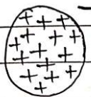
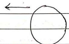
A (charged)
B (uncharged)
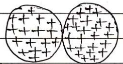
A(charged) B(charged)
By conduction
3) By induction method:
→ When a charged body is brought close to an uncharged body without touching,
charges are developed in the uncharged body. This method is called induction.
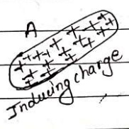
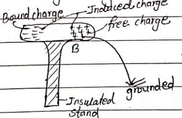
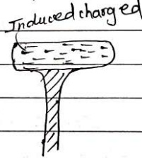
Fig:- charged body.
Fig.-charging a body by induction process.
When a charged object in (suppose a glass rod rubbed with silk) brings near to the uncharged object B which is mounted over an insulating stand then the negative charges of object B come closer towards the glass rod which is positively charged and positive charges of B towards goes towards the far end. Here negative charge of B are called Bound charge and because they are attracted by the positive charges of glass rod and positive charge of B is called free charge because they are away from the negative charges and able to move. If the far end of the object B is grounded by a conductor, then the free charges moves to the earth and object B becomes negatively charged object. In this way, an object is charged by induction method.
linear charge distribution:
It is one dimensional charge distribution. The charge distributed on a very thin straight rod is the linear charge distribution.
Linear charge density: The charge per unit length of a body is called linear charge density. It is denoted by \( \lambda \).
\( \therefore \lambda = \frac{q}{c} \rightarrow (1) \)
\( 5^{1/3}Si \) unit is \( cm^{-1} \).
Surface charge distribution:
→ It is two dimensional charge distribution. The charge distributed uniformly on a thin disc is the surface charge distribution.
Surface charge density: The charge per unit area of a body is called Surface charge density. It is denoted by \( \sigma \).
\( \therefore \sigma = \frac{q}{A} - \textcircled{11} \)
It is SI unit is \( cm^{-2} \).
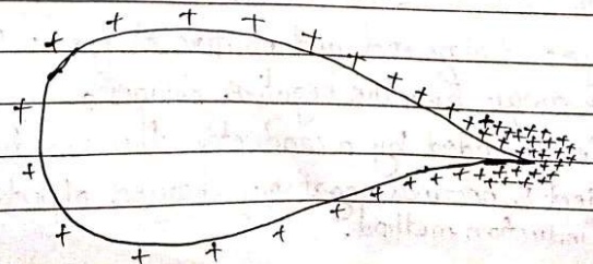
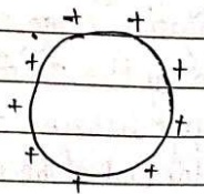
It has been found that the surface charge density depends upon the shape of the conductor. The charge spreads more i.e. the surface charge density is higher at sharp edges and corner. Some surface charge density distribution for various shapes of conductor can be shown as:
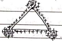
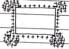
Action of point!
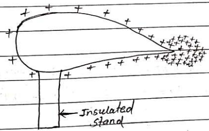
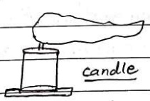
The density of charge on a conductor is very high at sharp edge or point on it. When the air particles come closer to the sharp point on a such a charged conductor, they get charge with similar polarity. The similarly charged air molecules are repelled and move away. Other uncharged molecules come to take the place of previous molecules and move away when they get charged. The process takes place continuously. As a result, it gives rise to the current of air called electric wind. This electric wind is enough to blow a candle placed near to it. This phenomenon is called action of point. During this process, the charged conductor continuously loosses its charge and finally becomes uncharged.
Electrostatic force
→ The charges interact with each other. It is found that same charges repell each other and opposite charges attract each other. These force of attraction and repulsion between charges at rest state is called electrostatic force.
Columb's law:-
This law states that, "The magnitude of force of attraction and repulsion between two charges is directly proportional to the product of their charges and inversely proportional to the square of the distance between them."
Consider two charges Q, and q_{2} placed at a distance r' apart from each other. Let F' be the electrostatic force between these charges then according to column's law,
The electrostatic force F' is:
(i) Directly proportional to the product of charges. i.e. \( f \propto q_{1} q_{2} \rightarrow 1 \)
(ii) Inversely proportional to the square of the distance between them.
1. e.e. \( F\alpha \frac{1}{\gamma^{2}} \) — (ii)
No. Combining eq(i) and eq(ii)
\( F\alpha\frac{q_{1}q_{2}}{r^{2}} \)
Here, 'k' is a proportionality constant and its value depends upon the nature of medium and also known the system of unit used in SI-units.
Here, \( k = \frac{1}{4\pi\varepsilon} \)
where, \( \varepsilon' \) is the permittivity of medium.
The electrostatic force \( F^{\prime} \) can be written as
\( \left| F = \frac{1}{4\pi\varepsilon} \frac{q_{1} q_{2}}{r^{2}} \right| \rightarrow \textcircled{3} \)
In SI unit, if \( q_{1} = q_{2} = xc \) and \( r = t_{m} \), in vacuum
Then, \( \frac{1}{4\pi\varepsilon} = g \times 10^{9} \)
and \( \varepsilon = 8.85 \times 10^{-12} \, C^{2} N^{-1} m^{-2} \)
Vacuum permittivity of medium is denoted by \( \varepsilon_{0} \) and electrostatic force becomes:
\( F = \frac{1}{4\pi\varepsilon_{0}} \frac{q_{1} q_{2}}{r^{2}} \) where, \( \frac{1}{4\pi\varepsilon_{0}} \approx 9 \times 10^{9} \)
Definition of permittivity of medium:
The permittivity of a medium can be defined as the response of the medium to the presence of an electrostatic force when a charges are placed in the medium. OR The ability of a medium to pass the electric charge through that medium is called permittivity of that medium.
Relative permittivity or dielectric constant ( \( \varepsilon_{r} \)):
The insulating materials which have also free electrons like metals are generally called dielectric. For constant Fox e.g.: mica, paper, wax, glass, etc.
The relative permittivity of a dielectric medium is defined as the ratio of permittivity of that medium to the permittivity of vacuum or free space. It is also called dielectric constant. It is denoted by \( \varepsilon_{r} \) and it is given as:
\( \varepsilon_{r}=\frac{\varepsilon}{\varepsilon_{0}} \)
\( or_{1} \), \( \varepsilon = \varepsilon_{r} \times \varepsilon_{0} \)
Again, the electrostatic force between 2 changes in a dielectric medium can be written as:
\( F=\frac{1}{4\pi\varepsilon_{r}\varepsilon_{0}}\frac{q_{1}q_{2}}{r^{2}} \)
Force due to multiple charges - electrostatic force due to multiple charges or a charge is equal to the vector sum of individual forces.
let \(q_{1}, q_{2}, q_{3}, q_{4}\) are the charges which exert electrostatic forces \(f_{1}, f_{2}, f_{3}\) and \(f_{4}\) on a given charge \(q\). Then the total electrostatic force on charge \(q\) can be written as:
$$f^{2} = f_{1} + f_{2} + f_{3} + f_{4}$$
Electrostatic field intensity or field strength ( \( \vec{E} \))
The space around the charge particle where the force of discharge particle can be experienced than the space or this region is called electric field.
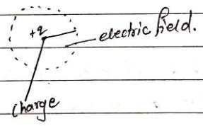
The electric intensity at a point in an electric field is defined as the force experienced by a unit positive test charge kept at that point. It is also known as electric field strength or simply electric field.
Electric field intensity is vector quantity. So, the field in terms of vector notation is:
It is also defined as force per unit charge at a point in the electric field.
Consider a charge q' placed where the electric field of the charge is shown in the diagram. Let a point A at a distance r from the charge, a unit positive charge placed at point A then the column's force between these two charges is given as:
$$ F=\frac{1}{4\pi\varepsilon_{0}}\frac{Q q}{r^{2}} $$
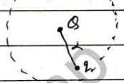
Here, \( q = +1c \)
$$ S_{0}. F = \frac{1}{4\pi\varepsilon_{0}} \frac{\cos}{r^{2}} = \overrightarrow{E} (Intensity) $$
$$ \therefore Hence, \overrightarrow{E} = \frac{1}{4\pi\varepsilon_{0}}\frac{\mathbf{Q}}{r^{2}} $$
This is the force exerted by charge Q at point A in the field. It is denoted by \( \overrightarrow{E} \), it is a vector quantity and the SI unit of electric field intensity ( \( \overrightarrow{E} \)) is N/columb. The direction of field intensity depends upon the nature of charge.
Electric field due to multiple charges!
→ Electric field intensity due to multiple charges is given by the vector sum of the electric field intensities at that point. If \( \overrightarrow{E}_{1}, \overrightarrow{E}_{2}, \overrightarrow{E}_{3} \ldots \overrightarrow{E}_{n} \) are the intensities at point A then the total intensities at that point can be written as:
\( \overrightarrow{F} = \overrightarrow{F} + \overrightarrow{F} + \overrightarrow{F}_{1} + \ldots + \overrightarrow{F}_{n} \)
→ It follows vector addition.
Electric lines of force:
Electric lines of forces are defined as the imaginary lines along which a unit positive charge moves if it is free to do so. It is also defined as the curve where the tangent at any point gives the direction of the electric field at that point.
Electric lines of forces are not the real lines drawn around the charge. These are the imaginary, infinite number of lines of force can be drawn around a point charge.
Properties of electric lines of force:
1) The electric lines of force start from positive charge and end to negative charge.
2) The electric lines of force do not intersect each other.
3) The tangent at any point on an electric lines of force gives the direction of electric field at that point.
4) The electric lines of force contract longitudinally due to attraction between unlike charges.
5) The lines of force exerted lateral pressure due to repulsion between like charges.
6) The lines of force do not pass through charged bodies.
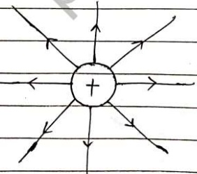
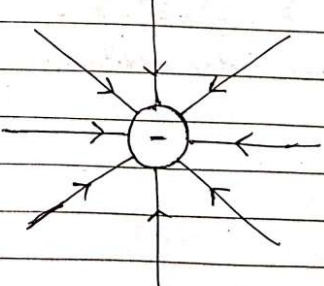
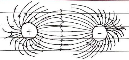
Fig: Attraction between opposite charges.
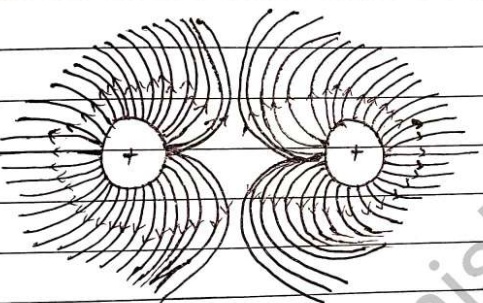
Fig.: Repulsion between same charges
Electric flux!
The total number of electric lines of force passing through an area is called
electric flux and denoted by \( \phi \).
It has been found that lines of forces are more close to each other in the region where electric field intensity is high. Thus, the number of electric lines of force (flux) passing through an area at a point is called a measure of the electric field intensity at that point.
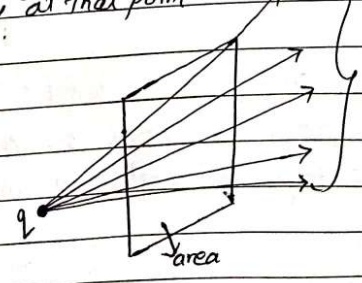
electric lines of force.
On the basis of electric lines of force, electric field intensity can also be defined as number of electric lines of force passing through unit area held perpendicular to the direction of line of force i.e.
## \( \overrightarrow{E}=\frac{\phi}{A} \)
\( \Phi=\overrightarrow{E\cdot A} \)
Mathematically, the scalar product of electric field ( \( \overrightarrow{E} \)) and area vector ( \( \overrightarrow{A} \)) is called electric field flux.
If \( \theta \) be the angle between \( \overrightarrow{E} \) and \( \overrightarrow{A} \), then we have,
\( \therefore \overrightarrow{\phi} = E A \cos \theta \)
The electric flux per unit area is called flux density.
The SI unit of electric flux is \( \sqrt{kgm^{3}s^{-3}A^{-1}} \) or \( \sqrt{Nm^{2}c^{-1}} \).
Grauss's Law in electrostatics.
It states that, "the total flux passing through any closed surface is enclosing a charge is equal to the \( \frac{1}{\varepsilon_{0}} \) times the charge enclosed by the closed surface (also called Gaussian's surface)"
i.e. Total electric flux \( (\phi) = \frac{1}{3} \times q \)
## \( \therefore \phi = \frac{2}{E_{0}} \)
Where, E is the permittivity of vacuum. The closed surface enclosing the charge may be of any shape and such surface are called Gaussian surface.
Flux due to a point charge (Proof of Gauss law)
Consider a point charge +q placed at a point '0'. Also consider a point
'p' at a distance 'r' from the charge and construct a sphere of radius 'r'.
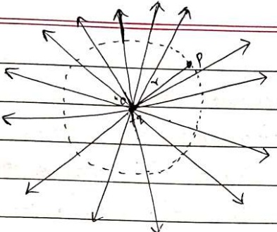
Here, the electric field intensity at point P is given as:
\( \overrightarrow{E} = \frac{1}{4\pi\varepsilon_{0}} \frac{q}{r^{2}} \)
Noo, The total lines of electric force passing through this area is given as:
From eqn(1) and eqn(ii).
\( a_{1} \) \( \Phi = \frac{1}{4\pi\varepsilon_{0}} \frac{q}{r^{2}} \). \( 4\pi r^{2} \) ( \( \because A = 4\pi r^{2} \))
$$ \cos\quad\phi=\frac{q}{\varepsilon_{0}} $$
$$ \therefore \phi = \frac{1}{\varepsilon_{0}} \times 2 $$
\( E q^{n}(3) \) verifies the Gauss law.
And, \( e q^{n}(3) \) is the flux due to point charge +q placed in vacuum which is \( \frac{1}{E_{0}} \) times of the given charge.
Here, the above relation is for vacuum medium and in SI unit.
Application of Grassis law:
(1) Electric field intensity due to charged sphere:
→ Consider a spherical body having radius R' contains charge +2.
Now, electric field intensity due to this charge, sphere is determined
at different points by using Gauss theorem as:
(a) Intensity at point 'p' on the surface of sphere:
→ let the point 'p' lie at the surface of the sphere having radius r'
and contains charge +q.
Consider a Gaussian surface passing through the point P' and endizes the charged sphere. Now, the electric flux passing through this Gaussian surface can be written as:
\( \phi = EA \)
\( \therefore \phi = E4\pi R^{2} - (i) \)
Also, From Gauss theorem,
\( \phi = \frac{q}{\varepsilon_{0}} \)
\( E_{1}H\pi R^{2}=\frac{q}{\varepsilon_{0}} \) (from ①)
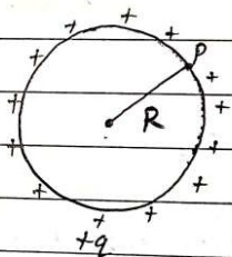
\( \therefore E=\frac{1}{4\pi R^{2}}\frac{q}{\varepsilon_{0}} \) —(1)
Eqn(ii) is the electric field intensity at point p which lie at the surface of sphere.
Intensity at point 'p' lie outside the sphere
let a point 'p' hit at a distance 'm'
from the charged sphere. Now
construct a surface through point 'p'
of radius (r) = R + m which encloses
the charged sphere.
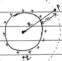
Now, The electric flux passing through this surface can be written as:
\( \Phi = EA \)
\( \therefore \Phi = E4\pi r^{2}-\Phi \) [where, \( r = R + n \)]
Applying laws theorem, The electric flux passing through this surface can be written as:
\( \phi = \frac{q}{\varepsilon_{0}} \)
\( \sigma_{1} \) \( E4\pi r^{2} = \frac{q}{\varepsilon_{0}} \)
\( \sigma_{1} \) \( E = \frac{q}{4\pi r^{2}\varepsilon_{0}} \)
\( \therefore E = \frac{1}{4\pi\varepsilon_{0}}\frac{q}{r^{2}} \) — ①
\( E_{n}(i) \) is the electric field intensity at point 'P' which lie outside the sphere.
Intensity at point p' lie at inside the sphere:
Consider a point 'P' inside the sphere at a distance 'm' from the surface of sphere. Now, imagine a surface having radius \( (R-n) \) which contain the point P. The electric flux at this sphere may be:
\( \phi = EA \)
\( \therefore \phi = E4\pi(R-n)^{2} \) —①
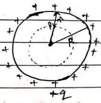
Applying laws theorem for this surface we have,
\( \phi = \frac{O}{\varepsilon_{0}} \)
or, \( E4\pi(R-n)^{2}=\frac{0}{\varepsilon_{0}} \)
\( \therefore E=0 \)
As we know that, the charge of a sphere distributed at the surface of sphere only. So, there is no any charge inside the sphere and the gaussian surface constructed with radius (R-n) donot encloses any charges.
Above relation shows that the electric field intensity inside the charged sphere is zero.
(2) Electric field intensity due to linear charged conductor:
→ Consider a linear charge conductor having uniform charge distribution, its linear charge density ( \( \lambda \)) given as:
\( \lambda = \frac{q}{L} \), where L is the length of conductor
Let a point \(P'\) at a distance \(r\) from the conductor
where electric field intensity is to be determined.
Consider a imaginary cylindrical surface of small
length \(L\) which contains the point \(P'\) Now, the
charge encloses throughout this surface can be written as
\(\therefore q = 2L - 1\)
The electric flux passing through this cylindrical surface
is given as:
\( \phi = EA \)
\( \therefore \phi = E2\pi r\ell - (ii) \)
According to Gauss's theorem, Electric flux passing through this surface is:
$$ \phi=\frac{q}{\varepsilon_{0}} $$
$$ \alpha_{1} \quad \Phi = \frac{\alpha \ell}{\varepsilon_{0}} \quad (from eq\text{①}) $$
$$ \text{or} \quad E2\pi r \bcancel{\ell } = \lambda \bcancel{\ell } \quad (from eq(ii)) $$
$$ \therefore \text{E} = \frac{\lambda}{2\pi r \varepsilon_{0}} $$
∴ This is the relation of electric field intensity at a point near the linear charged conductor.
③ Electric field intensity due to plane changed conductor.
Consider a plane charged conductor having uniform charge distribution and surface charge density (σ) of this plane charged conductor is given as:
\( \therefore \sigma = \frac{q}{2} - \frac{1}{2} \)
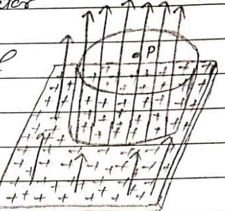
Consider, a point 'P' outside. Fig: showing plane charged conductor with electric lines of force.
the conductor Where electric field intensity is to be determined.
Construct a cylindrical shape having base area 'A' which contains the point 'P'.
The total electric flux passing through the base of cylindrical shape is given as:
\( \Phi = E A \) —(1)
\( \phi = EA \) —(ii)
Now, According to Gauss theorem, the electric flux passing through the cylinder is given as:
\( \phi = \frac{q}{\varepsilon_{0}} \rightarrow (ii) \)
from①, \( q = \sigma A \)
NaO, In eq \( ^{n} \)(iii),
\( \Phi=\frac{q}{\varepsilon_{0}} \)
\( a_{1}EA=\frac{6A}{\varepsilon_{0}} \) (From ① and \( q=\frac{6A}{1} \))
Eq(iv) is the relation for electric field intensity due to plane charged
is equal to the \( \frac{1}{E_{0}} \) times of \( \sigma \).
④ Electric field Intensity due to plane charged sheet:
→ Consider an inhile length plane sheet
with a uniform charge density ( \( \sigma \)).
Lel, 'p' be a point near to sheet
Where electric field intensity is to
be determined. For this consider
a small area 'A' surrounding
point 'P' with its plane parallel
to the sheet and construct cylindrical
gaussian surface whose walls are
perpendicular to the sheet, extending
by an equal distance on both sides of the
surface.
Fig. Electric field of plane charged
Sheet.
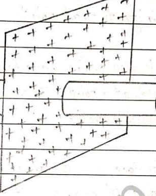
Total electrical flux passing through the two end flat faces is given as \( \phi = 2E \times A \xrightarrow{(i)} \)
According to Grauss theorem,
\( \phi = \frac{q}{\varepsilon_{0}} \rightarrow (1) \)
Here, \( q = \sigma A \), so above \( e a^{n} \) becomes,
\( \phi = \frac{\sigma A}{\varepsilon_{0}} \)
or, \( 2EA = \frac{\sigma A}{\varepsilon_{0}} \)
or, \( E = \frac{G A}{2 R E_{0}} \)
\( \therefore \sqrt{E} = \frac{6}{2 E_{0}} \) — (iii)
This is the formula for electric field intensity due to plane charged sheet.
Electric potential(V):
The electric potential at a point in electric field is defined as
amount of work done for bringing a unit positive charge from
infinity to that point.
It is also defined as the work done per unit charge due to electric field at a point. The SI unit of electric potential is Toute/column which is volt.
Consider a + Q charge placed at a point 'O' and a unit + re charge at point 'A' at a distance 'r' from the charge.
The electromagnetic force between both charge is given as \( \overrightarrow{F} = \frac{1}{4\pi\varepsilon_{0}} \frac{\varepsilon_{0} q}{r^{2}} \)
\( \overrightarrow{F} = \frac{1}{4\pi\varepsilon_{0}} \frac{\varepsilon_{0} q}{r^{2}} \)
\( a_{1} \) \( \overrightarrow{F}=\frac{1}{4\pi}\varepsilon_{0}\frac{Q}{r^{2}} \) \( \cdots \) (i)
This is also the intensity at point A due to charge \( q' \).
If the test charge brings a small distance, don against the
force. Then the work done can be written as:
NaO, The total work done for the bringing of unit +re charge can be obtained by integrating above equations over limits to r or
So, \( W = \int dw \)
$$ \alpha, \quad \omega = \int\limits_{\infty}^{x} - f \cdot d x $$
$$ a. W = \int\limits_\infty\frac{1}{4\pi\varepsilon_{0}}\frac{Q}{r^{2}} dr $$
$$ \alpha_{1} \quad W = -\frac{1}{4\pi\varepsilon_{0}}\frac{Q}{\bcancel{r}} \quad \int\limits_{\infty}^{r}\frac{1}{\gamma^{2}} d\gamma $$
$$ a, w = -\frac{Q}{4\pi\varepsilon_{0}}\int r^{2}dr $$
$$ \alpha, \quad \omega = -\frac{Q}{4\pi\varepsilon_{0}}\left[\frac{r^{-2+1}}{-2+1}\right]^{\gamma} $$
$$ \text{cr.} w = \frac{-Q}{4\pi\varepsilon_{0}} \left[ \frac{r^{-1}}{-1} \right] \infty $$
$$ \text{or}w=\frac{-Q}{4\pi\varepsilon_{0}}\left(\frac{r^{-1}}{-1}-\frac{\alpha^{-1}}{-1}\right) $$
$$ o r w=\frac{-Q}{4\pi\varepsilon_{0}}\left(-\frac{1}{r}\mp0\right) $$
$$ \therefore w = \frac{Q}{4\pi\varepsilon_{0}r} = \frac{1}{4\pi\varepsilon_{0}}\frac{q}{r} $$
This is the relation for electric potential at a point in the electric field. It is a scalar quantity.
Definition of I volt:
A point in an electric field is said to be had have I V of potential if
I go up of work is to be done in bringing I column of positive
charge from infinity to that point.
Definition of I stat column:
Electric potential energy:
The electric potential energy at a point in electric field is defined as the work done by bringing a charge from infinity to that point.
According to def of potential,
or \( W = \frac{1}{4\pi\varepsilon_{0}} \frac{Q}{r} \times q \)
\( W = \frac{82}{4\pi\varepsilon_{0}r} \)
This is the relation for electric potential energy.
Potential difference:
Consider a point A and B having distance r, and \( r_{2} \) from a point charge +8. The potential due to these charges at point A and B is given as:
\( V_{a} = \frac{1}{4\pi\varepsilon_{0}} \frac{Q}{r_{1}} \) and
\( V_{b} = \frac{1}{4\pi\varepsilon_{0}} \frac{Q}{r_{2}} \)
NaO, the difference in potential at point A to B can be determined as
$$ V_{ab} = \frac{1}{4\pi\varepsilon_{0}} \frac{\bcancel{Q}}{r_{1}} - \frac{1}{4\pi\varepsilon_{0}}\frac{\bcancel{Q}}{r_{2}} $$
This is the potential difference between point \( A' \) to \( B' \) due to given charge + Q.
Potential gradient \( \left(\frac{\Delta V}{\Delta t}\right) \):
The change in potential per unit length is defined as potential gradient. Let potential at a point due to a charge is given as:
\( \therefore V = \frac{1}{4\pi\varepsilon_{0}}\frac{Q}{r} \)
Now, According the def of potential gradient, we can written as:
\( \frac{dv}{dr} = \lim_{\Delta r \to 0} \frac{dv}{\Delta r} \)
Nano, differentiating potential with respect to distance (dr), the potential gradient can be obtained as
\( \frac{dv}{dr} = \frac{d\left(\frac{1}{4\pi\varepsilon_{0}}\frac{Q}{r}\right)}{dr} \)
\( \alpha_{r}\frac{dv}{dr}=\frac{Q}{4\pi\varepsilon_{0}}x-\pm x^{r^{-2}} \)
\( \therefore\frac{dv}{dr}=\frac{-Q}{4\pi\varepsilon_{0}r^{2}}=-E\Rightarrow E=\frac{dv}{dr} \)
Here, the electric field intensity can also be defined as negative of the potential gradient at a point.
Electron volt (ev):
To measure the energy of charge particles in joules will be
quit be large unit and hence inconvenient. Electron volt is the
unit of energy to represent the small energy of charge particles.
I electron volt of energy is defined as the energy gained by an electron when accelerated through potential difference of voltage. Here
Potential difference (pd) = \( \frac{\text{work done}}{\text{charge}} \)
work = p.d.x charge
for one electron void (ev),
\( p \cdot d = I \cdot v \cdot t \)
and charge = \( 1.6 \times 10^{-19} C \)
\( W = 1 \times 1.6 \times 10^{-19} \)
\( = 1.6 \times 10^{-19} \) joule
\( = 1 \text{ eV} \)
\( 1eV = 1.6 \times 10^{-19}J \)
Potential due to multiple charges:
Since, the electric potential is a scalar quantity, the total potential at a potential due to multiple charge is the algebraic sum of individual potential at that point.
Let, \( V_{1} \), \( V_{2} \) and \( V_{3} \) are the potential at point A due to
charges \( q_{1}, q_{2}, q_{3} \) respectively. Then, the total potential at point A can be written as:
\( V = V_{1} + V_{2} + V_{3} \)
Equipotential surface:
The surface on which the potential at which every point is same or there is no potential difference between any two points then the surface is called equipotential surface. For example: equipotential surface due to a charge can be represented by a diagram given as:
Fig.1: Showing equipotential surface Equip potential surfaces.